Programming is not just about programming languages, technologies and coding. It's mostly about thinking.
Learn to design, implement and optimize efficient algorithms using various basic techniques and simply start coding like a pro.
1. What makes a good programmer?
What's the difference between the programmer who can easily "nail" any coding interview, get job in any company including Google, NASA..., win any coding competition, and the others?
Is it how many programming languages he knows?
Is it how fast he types?
Is it how clean his code look?
Is it the one who can write a binary tree without surfing through Stakoverflow?
Well, maybe all of the above.
To me, however, one of the key traits of a good programmer is the ability to solve problems efficiently. The ability to analyse and understand the problem. The ability to design, implement and optimize the solution.
The truth is, not even decades of experience can guarantee that you will obtain these skills. What I want to achieve with this article is to introduce you to this problematic and motivate you to, instead of focusing on learning new languages and new technologies, focus on the efficiency of your solutions to given problems.
2. Motivational example
Let's say we are given a simple task to write a function that takes two parameters, format('truetype')%3Bfont-weight%3Anormal%3Bfont-style%3Anormal%3B%7D%3C%2Fstyle%3E%3C%2Fdefs%3E%3Ctext%20font-family%3D%22stix_italiced3d2c21991e3bef5e06%22%20font-size%3D%2216%22%20text-anchor%3D%22middle%22%20x%3D%224.5%22%20y%3D%2213%22%3Eb%3C%2Ftext%3E%3C%2Fsvg%3E) and
and format('truetype')%3Bfont-weight%3Anormal%3Bfont-style%3Anormal%3B%7D%3C%2Fstyle%3E%3C%2Fdefs%3E%3Ctext%20font-family%3D%22stix_italic38b3eff8baf56627478e%22%20font-size%3D%2216%22%20text-anchor%3D%22middle%22%20x%3D%223.5%22%20y%3D%2213%22%3Ee%3C%2Ftext%3E%3C%2Fsvg%3E) , and returns
, and returns format('truetype')%3Bfont-weight%3Anormal%3Bfont-style%3Anormal%3B%7D%3C%2Fstyle%3E%3C%2Fdefs%3E%3Ctext%20font-family%3D%22stix_italicbf07f8b6b55653dcdb52%22%20font-size%3D%2216%22%20text-anchor%3D%22middle%22%20x%3D%224.5%22%20y%3D%2216%22%3Eb%3C%2Ftext%3E%3Ctext%20font-family%3D%22stix_italicbf07f8b6b55653dcdb52%22%20font-size%3D%2212%22%20text-anchor%3D%22middle%22%20x%3D%2212.5%22%20y%3D%2210%22%3Ee%3C%2Ftext%3E%3C%2Fsvg%3E) (the power function).
(the power function).
For example format('truetype')%3Bfont-weight%3Anormal%3Bfont-style%3Anormal%3B%7D%3C%2Fstyle%3E%3C%2Fdefs%3E%3Ctext%20font-family%3D%22stixc8d639b8e18ef78818709734d36%22%20font-size%3D%2216%22%20text-anchor%3D%22middle%22%20x%3D%224.5%22%20y%3D%2218%22%3E2%3C%2Ftext%3E%3Ctext%20font-family%3D%22stixc8d639b8e18ef78818709734d36%22%20font-size%3D%2212%22%20text-anchor%3D%22middle%22%20x%3D%2212.5%22%20y%3D%2212%22%3E3%3C%2Ftext%3E%3Ctext%20font-family%3D%22stixc8d639b8e18ef78818709734d36%22%20font-size%3D%2216%22%20text-anchor%3D%22middle%22%20x%3D%2222.5%22%20y%3D%2218%22%3E%3D%3C%2Ftext%3E%3Ctext%20font-family%3D%22stixc8d639b8e18ef78818709734d36%22%20font-size%3D%2216%22%20text-anchor%3D%22middle%22%20x%3D%2234.5%22%20y%3D%2218%22%3E8%3C%2Ftext%3E%3C%2Fsvg%3E) .
.
Anyone with at least a little knowledge of programming should be able to come up with something like this:
Power(b, e):
Input: number b and number e
1.	result := 1
2.	while e > 0:
3.		result := result * b
4.		e := e - 1
Output: result
Equivalent C code would look like:
int power(int b, int e) {
    int result = 1;
    while (e > 0) {
        result *= b;
        e--;
    }
    return result;
}
Now we can run some tests to make sure it works correctly (check it our for yourself) and we are done. Great job! We solved the task, the code is clean and we can call ourselves good programmers.
But is it enough to work at Google or NASA? (both companies were taken as inspirational example since most would agree that that's where "good programmers" work)
Let's say our program is going to be used for calculations with a really large exponent . How fast is it going to be?
We can run some tests and measure the time. The following table is the result of running the code on an "average" CPU (2 GHz, single core).
| exponent size | running time |
|---|
| 10 | 0.000 ms |
| 100 | 0.001 ms |
| 1,000 | 0.005 ms |
| 10,000 | 0.047 ms |
| 100,000 | 0.460 ms |
| 1,000,000 | 4.610 ms |
| 10,000,000 | 46.02 ms |
| 100,000,000 | 460.1 ms |
| 1,000,000,000 | 4.599 s |
| 10,000,000,000 | 46.03 s |
As you can see, for small exponent, the calculation is relatively fast.
But for exponent being no more than 10 billion, the calculation already takes up to 46 seconds!
You may ask why would anyone need to calculate with an exponent that large in the first place.
What kind of real-world problems would require such calculation?
Well, have you ever visited a website through HTTPS protocol? (Literally any secured website like Google.com, Facebook.com, Youtube.com,...)
This protocol encrypts the communication between your device and the server using an algorithm called RSA.
And this algorithm, in order to work and to make the encryption secure, uses exponents as large as format('truetype')%3Bfont-weight%3Anormal%3Bfont-style%3Anormal%3B%7D%3C%2Fstyle%3E%3C%2Fdefs%3E%3Ctext%20font-family%3D%22stixce87a9d3432d0e13dcdb3ec4265%22%20font-size%3D%2216%22%20text-anchor%3D%22middle%22%20x%3D%224.5%22%20y%3D%2218%22%3E2%3C%2Ftext%3E%3Ctext%20font-family%3D%22stixce87a9d3432d0e13dcdb3ec4265%22%20font-size%3D%2212%22%20text-anchor%3D%22middle%22%20x%3D%2221.5%22%20y%3D%2212%22%3E1024%3C%2Ftext%3E%3C%2Fsvg%3E) which is:
which is:
179769313486231590772930519078902473361797697894230657273430081157732675805500963132708477322407536021120113879871393357658789768814416622492847430639474124377767893424865485276302219601246094119453082952085005768838150682342462881473913110540827237163350510684586298239947245938479716304835356329624224137216 (yep, seriously)
That's a lot more than 10 billion.
Now, how long would it take our program to calculate this?
Well, actually about
26220679155974177115376501096440077469105652437549804022029369712263132210735651293042265354882123385129230491497002808474057569426124536233017976657260471188471362567357065411705775780967419184256318934979598616351453396318816665993235782011512379843988420165065680556176536786006138473836151 years.
Which, by the way, is about
1748045277064945141025100073096005164607043495836653601468624647484208814049043419536151023658808225675282032766466853898270504628408302415534531777150698079231424171157137694113718385397827945617087928998639907756763559754587777732882385467434158656265894677671045370411769119067075 times the age of the universe.
And this calculation happens every time you visit or refresh a website. Can you imagine waiting that long for a website to load?
Fortunately, the people who designed RSA were good programmers and their algorithm can perform such calculation in a few milliseconds.
How do they do it? You will find out later in this article :-)
And hopefully by that time, you will be able to start coding efficiently like a good programmer yourself.
3. Complexity overview
In The basic concept of Algorithms article, you were introduced to algorithmic complexity analysis and something called Big-O notation.
Simply put, %3C%2Fmo%3E%3C%2Fmath%3E--%3E%3Cdefs%3E%3Cstyle%20type%3D%22text%2Fcss%22%3E%40font-face%7Bfont-family%3A'stix_italicd1fe173d08e959397adf'%3Bsrc%3Aurl(data%3Afont%2Ftruetype%3Bcharset%3Dutf-8%3Bbase64%2CAAEAAAAKAIAAAwAgT1MvMi7PBGUAAACsAAAATmNtYXCzVj0TAAAA%2FAAAADRnbHlmJRz6cgAAATAAAABlaGVhZAjbCH4AAAGYAAAANmhoZWEFzQfEAAAB0AAAACRobXR4MBdqngAAAfQAAAAIbG9jYQadRmQAAAH8AAAADG1heHAFYQCJAAACCAAAACBuYW1l%2FMdHqQAAAigAAAF7cG9zdAICAP8AAAOkAAAAIAAAAjsBkAAFAAAD6APoAAAAAAPoA%2BgAAAAAAAEA%2BgAAAAAAAAAAAAAAAAAAAAAAAAAAAAAAAAAAAAAgICAgAAAAINcbAwL%2FGgAAA%2F8BMQAAAAAAAgABAAEAAAAUAAMAAQAAABQABAAgAAAABAAEAAEAAABP%2F%2F8AAABP%2F%2F%2F%2FsgABAAAAAAACADz%2F7gK7ApsADwAfAAABFAYHBiMiJjU0Njc2MzYWBzQmIyIHDgEVFBYzMjc%2BAQK7c1xpbWN3Yk9wfWt2aUU8Y1c1PUM%2FXE47RgGia8Q%2BR3xuW8FFYQGGNEdRdUi2TlJXX0rWAAAAAAEAAAABAAAD7mBiXw889QADA%2Bj%2F%2F%2F%2F%2F0%2FxiZP%2F%2F%2F%2F%2FT%2FGJk%2FDb%2BzwWVA%2F8AAAAKAAIAAQAAAAAAAQAAA%2F%2F%2BzwAABcf8Nv4WBZUAAQAAAAAAAAAAAAAAAAAAAAIA%2BgAAAtIAPAAAAAAAAAAAAAAAZQABAAAAAgCGAAgAAAAAAAIAAAABAAEAAABAAAAAAAAAAAAAFQECAAAAAAAAAAEAFgAAAAAAAAAAAAIADgAWAAAAAAAAAAMAGAAkAAAAAAAAAAQAFgA8AAAAAAAAAAUAHABSAAAAAAAAAAYACwBuAAAAAAAAAAgAAAB5AAEAAAAAAAEAFgAAAAEAAAAAAAIADgAWAAEAAAAAAAMAGAAkAAEAAAAAAAQAFgA8AAEAAAAAAAUAHABSAAEAAAAAAAYACwBuAAEAAAAAAAgAAAB5AAMAAQQJAAEAFgAAAAMAAQQJAAIADgAWAAMAAQQJAAMAGAAkAAMAAQQJAAQAFgA8AAMAAQQJAAUAHABSAAMAAQQJAAYACwBuAAMAAQQJAAgAAAB5AFMAVABJAFgALQBJAHQAYQBsAGkAYwBSAGUAZwB1AGwAYQByACAAUwBUAEkAWAAtAEkAdABhAGwAaQBjAFMAVABJAFgALQBJAHQAYQBsAGkAYwBWAGUAcgBzAGkAbwBuACAAMQAuADEALgAxACBTVElYLUl0YWxpYwAAAwAAAAAAAAH%2FAP8AAAAAAAAAAAAAAAAAAAAAAAAAAA%3D%3D)format('truetype')%3Bfont-weight%3Anormal%3Bfont-style%3Anormal%3B%7D%40font-face%7Bfont-family%3A'stix9f92a457f2409ba2be014494216'%3Bsrc%3Aurl(data%3Afont%2Ftruetype%3Bcharset%3Dutf-8%3Bbase64%2CAAEAAAANAIAAAwBQT1MvMi8nBU0AAADcAAAATmNtYXDCjdaBAAABLAAAADxjdnQgSG4BcAAAAWgAAADYZnBnbUUgjnwAAAJAAAANbWdseWYcKO%2BSAAAPsAAAAHJoZWFkDLPdGwAAECQAAAA2aGhlYQjYEyQAABBcAAAAJGhtdHg0LeORAAAQgAAAAAxsb2NhTQ9wLwAAEIwAAAAQbWF4cBlhFX0AABCcAAAAIG5hbWV4T00CAAAQvAAAAZ5wb3N0AgIA%2FwAAElwAAAAgcHJlcFWzoI8AABJ8AAAAvAAAApwBkAAFAAAD6APoAAAAAAPoA%2BgAAAAAAAEA%2BgAAAAAAAAAAAAAAAAAAAAAAAAAAAAAAAAAAAAAgICAgAAAAINf%2FAqX%2BvQAAA%2F8B5gAAAAAAAgABAAEAAAAUAAMAAQAAABQABAAoAAAABgAEAAEAAgAoACn%2F%2FwAAACgAKf%2F%2F%2F9n%2F2QABAAAAAAAAAAAAAAAAAAAAAAAAAAAAAAAAAAAAAAAAAAAAAAAAAAAAAAAAAAAAAAAAAAAAWgBaABwAHAKWAAABwgAA%2FycD%2F%2F4aAqT%2F8gHM%2F%2Fb%2FJgP%2F%2FhoAWQBZACAAIAKWAAACqwHC%2F%2Fb%2FJwP%2F%2FhoCpP%2FyAqsBzP%2F2%2FyYD%2F%2F4aAFoAWgAcABwClgAAAqsBwgAA%2FycD%2F%2F4aAqT%2F8gKrAcz%2F9v8mA%2F%2F%2BGgBaAFoAHAAcApYBDgKrAjoBUP%2FsA%2F%2F%2BGgKk%2F%2FICqwI6%2F%2Fb%2F7AP%2F%2FhoAGAAYABgAGAP%2F%2FhoD%2F%2F4asAAsILAAVVhFWSAgS7gADlFLsAZTWliwNBuwKFlgZiCKVViwAiVhuQgACABjYyNiGyEhsABZsABDI0SyAAEAQ2BCLbABLLAgYGYtsAIsIGQgsMBQsAQmWrIoAQtDRWNFsAZFWCGwAyVZUltYISMhG4pYILBQUFghsEBZGyCwOFBYIbA4WVkgsQELQ0VjRWFksChQWCGxAQtDRWNFILAwUFghsDBZGyCwwFBYIGYgiophILAKUFhgGyCwIFBYIbAKYBsgsDZQWCGwNmAbYFlZWRuwAiWwCkNjsABSWLAAS7AKUFghsApDG0uwHlBYIbAeS2G4EABjsApDY7gFAGJZWWRhWbABK1lZI7AAUFhlWVktsAMsIEUgsAQlYWQgsAVDUFiwBSNCsAYjQhshIVmwAWAtsAQsIyEjISBksQViQiCwBiNCsAZFWBuxAQtDRWOxAQtDsAVgRWOwAyohILAGQyCKIIqwASuxMAUlsAQmUVhgUBthUllYI1khWSCwQFNYsAErGyGwQFkjsABQWGVZLbAFLLAHQyuyAAIAQ2BCLbAGLLAHI0IjILAAI0JhsAJiZrABY7ABYLAFKi2wBywgIEUgsAxDY7gEAGIgsABQWLBAYFlmsAFjYESwAWAtsAgssgcMAENFQiohsgABAENgQi2wCSywAEMjRLIAAQBDYEItsAosICBFILABKyOwAEOwBCVgIEWKI2EgZCCwIFBYIbAAG7AwUFiwIBuwQFlZI7AAUFhlWbADJSNhRESwAWAtsAssICBFILABKyOwAEOwBCVgIEWKI2EgZLAkUFiwABuwQFkjsABQWGVZsAMlI2FERLABYC2wDCwgsAAjQrILCgNFWCEbIyFZKiEtsA0ssQICRbBkYUQtsA4ssAFgICCwDUNKsABQWCCwDSNCWbAOQ0qwAFJYILAOI0JZLbAPLCCwEGJmsAFjILgEAGOKI2GwD0NgIIpgILAPI0IjLbAQLEtUWLEEZERZJLANZSN4LbARLEtRWEtTWLEEZERZGyFZJLATZSN4LbASLLEAEENVWLEQEEOwAWFCsA8rWbAAQ7ACJUKxDQIlQrEOAiVCsAEWIyCwAyVQWLEBAENgsAQlQoqKIIojYbAOKiEjsAFhIIojYbAOKiEbsQEAQ2CwAiVCsAIlYbAOKiFZsA1DR7AOQ0dgsAJiILAAUFiwQGBZZrABYyCwDENjuAQAYiCwAFBYsEBgWWawAWNgsQAAEyNEsAFDsAA%2BsgEBAUNgQi2wEywAsQACRVRYsBAjQiBFsAwjQrALI7AFYEIgYLABYbUSEgEADwBCQopgsRIGK7CJKxsiWS2wFCyxABMrLbAVLLEBEystsBYssQITKy2wFyyxAxMrLbAYLLEEEystsBkssQUTKy2wGiyxBhMrLbAbLLEHEystsBwssQgTKy2wHSyxCRMrLbApLCMgsBBiZrABY7AGYEtUWCMgLrABXRshIVktsCosIyCwEGJmsAFjsBZgS1RYIyAusAFxGyEhWS2wKywjILAQYmawAWOwJmBLVFgjIC6wAXIbISFZLbAeLACwDSuxAAJFVFiwECNCIEWwDCNCsAsjsAVgQiBgsAFhtRISAQAPAEJCimCxEgYrsIkrGyJZLbAfLLEAHistsCAssQEeKy2wISyxAh4rLbAiLLEDHistsCMssQQeKy2wJCyxBR4rLbAlLLEGHistsCYssQceKy2wJyyxCB4rLbAoLLEJHistsCwsIDywAWAtsC0sIGCwEmAgQyOwAWBDsAIlYbABYLAsKiEtsC4ssC0rsC0qLbAvLCAgRyAgsAxDY7gEAGIgsABQWLBAYFlmsAFjYCNhOCMgilVYIEcgILAMQ2O4BABiILAAUFiwQGBZZrABY2AjYTgbIVktsDAsALEAAkVUWLEMC0VCsAEWsC8qsQUBFUVYMFkbIlktsDEsALANK7EAAkVUWLEMC0VCsAEWsC8qsQUBFUVYMFkbIlktsDIsIDWwAWAtsDMsALEMC0VCsAFFY7gEAGIgsABQWLBAYFlmsAFjsAErsAxDY7gEAGIgsABQWLBAYFlmsAFjsAErsAAWtAAAAAAARD4jOLEyARUqIS2wNCwgPCBHILAMQ2O4BABiILAAUFiwQGBZZrABY2CwAENhOC2wNSwuFzwtsDYsIDwgRyCwDENjuAQAYiCwAFBYsEBgWWawAWNgsABDYbABQ2M4LbA3LLECABYlIC4gR7AAI0KwAiVJiopHI0cjYSBYYhshWbABI0KyNgEBFRQqLbA4LLAAFrARI0KwBCWwBCVHI0cjYbEKAEKwCUMrZYouIyAgPIo4LbA5LLAAFrARI0KwBCWwBCUgLkcjRyNhILAEI0KxCgBCsAlDKyCwYFBYILBAUVizAiADIBuzAiYDGllCQiMgsAhDIIojRyNHI2EjRmCwBEOwAmIgsABQWLBAYFlmsAFjYCCwASsgiophILACQ2BkI7ADQ2FkUFiwAkNhG7ADQ2BZsAMlsAJiILAAUFiwQGBZZrABY2EjICCwBCYjRmE4GyOwCENGsAIlsAhDRyNHI2FgILAEQ7ACYiCwAFBYsEBgWWawAWNgIyCwASsjsARDYLABK7AFJWGwBSWwAmIgsABQWLBAYFlmsAFjsAQmYSCwBCVgZCOwAyVgZFBYIRsjIVkjICCwBCYjRmE4WS2wOiywABawESNCICAgsAUmIC5HI0cjYSM8OC2wOyywABawESNCILAII0IgICBGI0ewASsjYTgtsDwssAAWsBEjQrADJbACJUcjRyNhsABUWC4gPCMhG7ACJbACJUcjRyNhILAFJbAEJUcjRyNhsAYlsAUlSbACJWG5CAAIAGNjIyBYYhshWWO4BABiILAAUFiwQGBZZrABY2AjLiMgIDyKOCMhWS2wPSywABawESNCILAIQyAuRyNHI2EgYLAgYGawAmIgsABQWLBAYFlmsAFjIyAgPIo4LbA%2BLCMgLkawAiVGsBFDWFAbUllYIDxZLrEuARQrLbA%2FLCMgLkawAiVGsBFDWFIbUFlYIDxZLrEuARQrLbBALCMgLkawAiVGsBFDWFAbUllYIDxZIyAuRrACJUawEUNYUhtQWVggPFkusS4BFCstsEEssDgrIyAuRrACJUawEUNYUBtSWVggPFkusS4BFCstsEIssDkriiAgPLAEI0KKOCMgLkawAiVGsBFDWFAbUllYIDxZLrEuARQrsARDLrAuKy2wQyywABawBCWwBCYgICBGI0dhsAojQi5HI0cjYbAJQysjIDwgLiM4sS4BFCstsEQssQgEJUKwABawBCWwBCUgLkcjRyNhILAEI0KxCgBCsAlDKyCwYFBYILBAUVizAiADIBuzAiYDGllCQiMgR7AEQ7ACYiCwAFBYsEBgWWawAWNgILABKyCKimEgsAJDYGQjsANDYWRQWLACQ2EbsANDYFmwAyWwAmIgsABQWLBAYFlmsAFjYbACJUZhOCMgPCM4GyEgIEYjR7ABKyNhOCFZsS4BFCstsEUssQA4Ky6xLgEUKy2wRiyxADkrISMgIDywBCNCIzixLgEUK7AEQy6wListsEcssAAVIEewACNCsgABARUUEy6wNCotsEgssAAVIEewACNCsgABARUUEy6wNCotsEkssQABFBOwNSotsEossDcqLbBLLLAAFkUjIC4gRoojYTixLgEUKy2wTCywCCNCsEsrLbBNLLIAAEQrLbBOLLIAAUQrLbBPLLIBAEQrLbBQLLIBAUQrLbBRLLIAAEUrLbBSLLIAAUUrLbBTLLIBAEUrLbBULLIBAUUrLbBVLLMAAABBKy2wViyzAAEAQSstsFcsswEAAEErLbBYLLMBAQBBKy2wWSyzAAABQSstsFosswABAUErLbBbLLMBAAFBKy2wXCyzAQEBQSstsF0ssgAAQystsF4ssgABQystsF8ssgEAQystsGAssgEBQystsGEssgAARistsGIssgABRistsGMssgEARistsGQssgEBRistsGUsswAAAEIrLbBmLLMAAQBCKy2wZyyzAQAAQistsGgsswEBAEIrLbBpLLMAAAFCKy2waiyzAAEBQistsGssswEAAUIrLbBsLLMBAQFCKy2wbSyxADorLrEuARQrLbBuLLEAOiuwPistsG8ssQA6K7A%2FKy2wcCywABaxADorsEArLbBxLLEBOiuwPistsHIssQE6K7A%2FKy2wcyywABaxATorsEArLbB0LLEAOysusS4BFCstsHUssQA7K7A%2BKy2wdiyxADsrsD8rLbB3LLEAOyuwQCstsHgssQE7K7A%2BKy2weSyxATsrsD8rLbB6LLEBOyuwQCstsHsssQA8Ky6xLgEUKy2wfCyxADwrsD4rLbB9LLEAPCuwPystsH4ssQA8K7BAKy2wfyyxATwrsD4rLbCALLEBPCuwPystsIEssQE8K7BAKy2wgiyxAD0rLrEuARQrLbCDLLEAPSuwPistsIQssQA9K7A%2FKy2whSyxAD0rsEArLbCGLLEBPSuwPistsIcssQE9K7A%2FKy2wiCyxAT0rsEArLbCJLLMJBAIDRVghGyMhWUIrsAhlsAMkUHixBQEVRVgwWS0AAAAAAQAw%2F08BMAKkAAwABrMGAQEwKwUHLgE1EDcXDgEVFBYBMAx0gPcJZkRGoRBC6IMBFZMQV6mVlLgAAQAd%2F08BHQKkAAwABrMGAQEwKxM3HgEVEAcnPgE1NCYdDHKC9wlnQ0MClBBE6IH%2B75cQVamXmLcAAAABAAAAAQAAM5ipa18PPPUAAwPo%2F%2F%2F%2F%2F9RjTQ3%2F%2F%2F%2F%2F1GNNDfw2%2FhoIoAP%2FAAAACgACAAEAAAAAAAEAAAP%2F%2FhoAAAj4%2FDb9yQigAAEAAAAAAAAAAAAAAAAAAAADAPoAAAFNADABTQAdAAAAAAAAAAAAAAA5AAAAcgABAAAAAwcMAS0AAAAAAAIDiAOaAIsAAAXYCtUAAAAAAAAAFQECAAAAAAAAAAEAIAAAAAAAAAAAAAIADgAgAAAAAAAAAAMAIgAuAAAAAAAAAAQAIABQAAAAAAAAAAUAHABwAAAAAAAAAAYAEACMAAAAAAAAAAgAAACcAAEAAAAAAAEAIAAAAAEAAAAAAAIADgAgAAEAAAAAAAMAIgAuAAEAAAAAAAQAIABQAAEAAAAAAAUAHABwAAEAAAAAAAYAEACMAAEAAAAAAAgAAACcAAMAAQQJAAEAIAAAAAMAAQQJAAIADgAgAAMAAQQJAAMAIgAuAAMAAQQJAAQAIABQAAMAAQQJAAUAHABwAAMAAQQJAAYAEACMAAMAAQQJAAgAAACcAFMAVABJAFgALQBSAGUAZwB1AGwAYQByAC0AVABUAEYAUgBlAGcAdQBsAGEAcgAgAFMAVABJAFgALQBSAGUAZwB1AGwAYQByAC0AVABUAEYAUwBUAEkAWAAtAFIAZQBnAHUAbABhAHIALQBUAFQARgBWAGUAcgBzAGkAbwBuACAAMQAuADEALgAxACBTVElYLVJlZ3VsYXItVFRGAAAAAwAAAAAAAAH%2FAP8AAAAAAAAAAAAAAAAAAAAAAAAAAABLuADIUlixAQGOWbABuQgACABjcLEAB0K2AF9LNyMFACqxAAdCQAxmAlIIPggqCBgHBQgqsQAHQkAMagBcBkgGNAYhBQUIKrEADEK%2BGcAUwA%2FACsAGQAAFAAkqsQARQr4AQABAAEAAQABAAAUACSqxAwBEsSQBiFFYsECIWLEDAESxJgGIUVi6CIAAAQRAiGNUWLEDAERZWVlZQAxoAlQIQAgsCBoHBQwquAH%2FhbAEjbECAESzBWQGAERE)format('truetype')%3Bfont-weight%3Anormal%3Bfont-style%3Anormal%3B%7D%3C%2Fstyle%3E%3C%2Fdefs%3E%3Ctext%20font-family%3D%22stix_italicd1fe173d08e959397adf%22%20font-size%3D%2216%22%20text-anchor%3D%22middle%22%20x%3D%226.5%22%20y%3D%2216%22%3EO%3C%2Ftext%3E%3Ctext%20font-family%3D%22stix9f92a457f2409ba2be014494216%22%20font-size%3D%2216%22%20text-anchor%3D%22middle%22%20x%3D%2217.5%22%20y%3D%2216%22%3E(%3C%2Ftext%3E%3Ctext%20font-family%3D%22stix9f92a457f2409ba2be014494216%22%20font-size%3D%2216%22%20text-anchor%3D%22middle%22%20x%3D%2225.5%22%20y%3D%2216%22%3E)%3C%2Ftext%3E%3C%2Fsvg%3E) describes how (asymptotically) efficient is our algorithm in worst-case in relation to
describes how (asymptotically) efficient is our algorithm in worst-case in relation to format('truetype')%3Bfont-weight%3Anormal%3Bfont-style%3Anormal%3B%7D%3C%2Fstyle%3E%3C%2Fdefs%3E%3Ctext%20font-family%3D%22stix_italic5f93f983524def3dca46%22%20font-size%3D%2216%22%20text-anchor%3D%22middle%22%20x%3D%224.5%22%20y%3D%2214%22%3En%3C%2Ftext%3E%3C%2Fsvg%3E) , which stands for the size of data our algorithm works with.
, which stands for the size of data our algorithm works with.
I will just put a table that sums up the general asymptotic functions we use in Big-O notation and their approximate running time here (considering 1 operation takes 1 ns):
From this table we should be able to determine which complexity we should aim for depending on the expected input size.
For example, if we are to build an algorithm on a database of hundreds of records, it should be fine if we come up with anything more efficient than exponential complexity.
Similarly, if we want to build an algorithm on a large data set of, let's say, billions of records, we should definitely aim for as efficient algorithm as possible.
We also have some other notions:
- worst-case complexity (the algorithm will never be slower than this)
%3C%2Fmo%3E%3C%2Fmath%3E--%3E%3Cdefs%3E%3Cstyle%20type%3D%22text%2Fcss%22%3E%40font-face%7Bfont-family%3A'stix_italic6d0f846348a856321729'%3Bsrc%3Aurl(data%3Afont%2Ftruetype%3Bcharset%3Dutf-8%3Bbase64%2CAAEAAAAKAIAAAwAgT1MvMi7PBGUAAACsAAAATmNtYXCzVj0TAAAA%2FAAAADRnbHlmJRz6cgAAATAAAACZaGVhZAjbCH4AAAHMAAAANmhoZWEFzQfEAAACBAAAACRobXR4MBdqngAAAigAAAAIbG9jYQadRmQAAAIwAAAADG1heHAFYQCJAAACPAAAACBuYW1l%2FMdHqQAAAlwAAAF7cG9zdAICAP8AAAPYAAAAIAAAAjsBkAAFAAAD6APoAAAAAAPoA%2BgAAAAAAAEA%2BgAAAAAAAAAAAAAAAAAAAAAAAAAAAAAAAAAAAAAgICAgAAAAINcbAwL%2FGgAAA%2F8BMQAAAAAAAgABAAEAAAAUAAMAAQAAABQABAAgAAAABAAEAAEAAAOY%2F%2F8AAAOY%2F%2F%2F8aQABAAAAAAADADz%2F7gK7ApsAFAAkADQAAAEzBhUjNCYrASIHIzY1Mx4BOwEyNjcUBgcGIyImNTQ2NzYzNhYHNCYjIgcOARUUFjMyNz4BAgwTNRMVGmk8GBM1EwYUGmIdMrZzXGlxY3NiT3B9a3ZpRTxjVzU9Qz9cTjtGAa2JSCAaOoFQIxYeEGvEPkd7b1vBRWEBhjRHUXVItk5SV19K1gAAAAABAAAAAQAAA%2B5gYl8PPPUAAwPo%2F%2F%2F%2F%2F9P8YmT%2F%2F%2F%2F%2F0%2FxiZPw2%2Fs8FlQP%2FAAAACgACAAEAAAAAAAEAAAP%2F%2Fs8AAAXH%2FDb%2BFgWVAAEAAAAAAAAAAAAAAAAAAAACAPoAAALSADwAAAAAAAAAAAAAAJkAAQAAAAIAhgAIAAAAAAACAAAAAQABAAAAQAAAAAAAAAAAABUBAgAAAAAAAAABABYAAAAAAAAAAAACAA4AFgAAAAAAAAADABgAJAAAAAAAAAAEABYAPAAAAAAAAAAFABwAUgAAAAAAAAAGAAsAbgAAAAAAAAAIAAAAeQABAAAAAAABABYAAAABAAAAAAACAA4AFgABAAAAAAADABgAJAABAAAAAAAEABYAPAABAAAAAAAFABwAUgABAAAAAAAGAAsAbgABAAAAAAAIAAAAeQADAAEECQABABYAAAADAAEECQACAA4AFgADAAEECQADABgAJAADAAEECQAEABYAPAADAAEECQAFABwAUgADAAEECQAGAAsAbgADAAEECQAIAAAAeQBTAFQASQBYAC0ASQB0AGEAbABpAGMAUgBlAGcAdQBsAGEAcgAgAFMAVABJAFgALQBJAHQAYQBsAGkAYwBTAFQASQBYAC0ASQB0AGEAbABpAGMAVgBlAHIAcwBpAG8AbgAgADEALgAxAC4AMQAgU1RJWC1JdGFsaWMAAAMAAAAAAAAB%2FwD%2FAAAAAAAAAAAAAAAAAAAAAAAAAAA%3D)format('truetype')%3Bfont-weight%3Anormal%3Bfont-style%3Anormal%3B%7D%40font-face%7Bfont-family%3A'stix9f92a457f2409ba2be014494216'%3Bsrc%3Aurl(data%3Afont%2Ftruetype%3Bcharset%3Dutf-8%3Bbase64%2CAAEAAAANAIAAAwBQT1MvMi8nBU0AAADcAAAATmNtYXDCjdaBAAABLAAAADxjdnQgSG4BcAAAAWgAAADYZnBnbUUgjnwAAAJAAAANbWdseWYcKO%2BSAAAPsAAAAHJoZWFkDLPdGwAAECQAAAA2aGhlYQjYEyQAABBcAAAAJGhtdHg0LeORAAAQgAAAAAxsb2NhTQ9wLwAAEIwAAAAQbWF4cBlhFX0AABCcAAAAIG5hbWV4T00CAAAQvAAAAZ5wb3N0AgIA%2FwAAElwAAAAgcHJlcFWzoI8AABJ8AAAAvAAAApwBkAAFAAAD6APoAAAAAAPoA%2BgAAAAAAAEA%2BgAAAAAAAAAAAAAAAAAAAAAAAAAAAAAAAAAAAAAgICAgAAAAINf%2FAqX%2BvQAAA%2F8B5gAAAAAAAgABAAEAAAAUAAMAAQAAABQABAAoAAAABgAEAAEAAgAoACn%2F%2FwAAACgAKf%2F%2F%2F9n%2F2QABAAAAAAAAAAAAAAAAAAAAAAAAAAAAAAAAAAAAAAAAAAAAAAAAAAAAAAAAAAAAAAAAAAAAWgBaABwAHAKWAAABwgAA%2FycD%2F%2F4aAqT%2F8gHM%2F%2Fb%2FJgP%2F%2FhoAWQBZACAAIAKWAAACqwHC%2F%2Fb%2FJwP%2F%2FhoCpP%2FyAqsBzP%2F2%2FyYD%2F%2F4aAFoAWgAcABwClgAAAqsBwgAA%2FycD%2F%2F4aAqT%2F8gKrAcz%2F9v8mA%2F%2F%2BGgBaAFoAHAAcApYBDgKrAjoBUP%2FsA%2F%2F%2BGgKk%2F%2FICqwI6%2F%2Fb%2F7AP%2F%2FhoAGAAYABgAGAP%2F%2FhoD%2F%2F4asAAsILAAVVhFWSAgS7gADlFLsAZTWliwNBuwKFlgZiCKVViwAiVhuQgACABjYyNiGyEhsABZsABDI0SyAAEAQ2BCLbABLLAgYGYtsAIsIGQgsMBQsAQmWrIoAQtDRWNFsAZFWCGwAyVZUltYISMhG4pYILBQUFghsEBZGyCwOFBYIbA4WVkgsQELQ0VjRWFksChQWCGxAQtDRWNFILAwUFghsDBZGyCwwFBYIGYgiophILAKUFhgGyCwIFBYIbAKYBsgsDZQWCGwNmAbYFlZWRuwAiWwCkNjsABSWLAAS7AKUFghsApDG0uwHlBYIbAeS2G4EABjsApDY7gFAGJZWWRhWbABK1lZI7AAUFhlWVktsAMsIEUgsAQlYWQgsAVDUFiwBSNCsAYjQhshIVmwAWAtsAQsIyEjISBksQViQiCwBiNCsAZFWBuxAQtDRWOxAQtDsAVgRWOwAyohILAGQyCKIIqwASuxMAUlsAQmUVhgUBthUllYI1khWSCwQFNYsAErGyGwQFkjsABQWGVZLbAFLLAHQyuyAAIAQ2BCLbAGLLAHI0IjILAAI0JhsAJiZrABY7ABYLAFKi2wBywgIEUgsAxDY7gEAGIgsABQWLBAYFlmsAFjYESwAWAtsAgssgcMAENFQiohsgABAENgQi2wCSywAEMjRLIAAQBDYEItsAosICBFILABKyOwAEOwBCVgIEWKI2EgZCCwIFBYIbAAG7AwUFiwIBuwQFlZI7AAUFhlWbADJSNhRESwAWAtsAssICBFILABKyOwAEOwBCVgIEWKI2EgZLAkUFiwABuwQFkjsABQWGVZsAMlI2FERLABYC2wDCwgsAAjQrILCgNFWCEbIyFZKiEtsA0ssQICRbBkYUQtsA4ssAFgICCwDUNKsABQWCCwDSNCWbAOQ0qwAFJYILAOI0JZLbAPLCCwEGJmsAFjILgEAGOKI2GwD0NgIIpgILAPI0IjLbAQLEtUWLEEZERZJLANZSN4LbARLEtRWEtTWLEEZERZGyFZJLATZSN4LbASLLEAEENVWLEQEEOwAWFCsA8rWbAAQ7ACJUKxDQIlQrEOAiVCsAEWIyCwAyVQWLEBAENgsAQlQoqKIIojYbAOKiEjsAFhIIojYbAOKiEbsQEAQ2CwAiVCsAIlYbAOKiFZsA1DR7AOQ0dgsAJiILAAUFiwQGBZZrABYyCwDENjuAQAYiCwAFBYsEBgWWawAWNgsQAAEyNEsAFDsAA%2BsgEBAUNgQi2wEywAsQACRVRYsBAjQiBFsAwjQrALI7AFYEIgYLABYbUSEgEADwBCQopgsRIGK7CJKxsiWS2wFCyxABMrLbAVLLEBEystsBYssQITKy2wFyyxAxMrLbAYLLEEEystsBkssQUTKy2wGiyxBhMrLbAbLLEHEystsBwssQgTKy2wHSyxCRMrLbApLCMgsBBiZrABY7AGYEtUWCMgLrABXRshIVktsCosIyCwEGJmsAFjsBZgS1RYIyAusAFxGyEhWS2wKywjILAQYmawAWOwJmBLVFgjIC6wAXIbISFZLbAeLACwDSuxAAJFVFiwECNCIEWwDCNCsAsjsAVgQiBgsAFhtRISAQAPAEJCimCxEgYrsIkrGyJZLbAfLLEAHistsCAssQEeKy2wISyxAh4rLbAiLLEDHistsCMssQQeKy2wJCyxBR4rLbAlLLEGHistsCYssQceKy2wJyyxCB4rLbAoLLEJHistsCwsIDywAWAtsC0sIGCwEmAgQyOwAWBDsAIlYbABYLAsKiEtsC4ssC0rsC0qLbAvLCAgRyAgsAxDY7gEAGIgsABQWLBAYFlmsAFjYCNhOCMgilVYIEcgILAMQ2O4BABiILAAUFiwQGBZZrABY2AjYTgbIVktsDAsALEAAkVUWLEMC0VCsAEWsC8qsQUBFUVYMFkbIlktsDEsALANK7EAAkVUWLEMC0VCsAEWsC8qsQUBFUVYMFkbIlktsDIsIDWwAWAtsDMsALEMC0VCsAFFY7gEAGIgsABQWLBAYFlmsAFjsAErsAxDY7gEAGIgsABQWLBAYFlmsAFjsAErsAAWtAAAAAAARD4jOLEyARUqIS2wNCwgPCBHILAMQ2O4BABiILAAUFiwQGBZZrABY2CwAENhOC2wNSwuFzwtsDYsIDwgRyCwDENjuAQAYiCwAFBYsEBgWWawAWNgsABDYbABQ2M4LbA3LLECABYlIC4gR7AAI0KwAiVJiopHI0cjYSBYYhshWbABI0KyNgEBFRQqLbA4LLAAFrARI0KwBCWwBCVHI0cjYbEKAEKwCUMrZYouIyAgPIo4LbA5LLAAFrARI0KwBCWwBCUgLkcjRyNhILAEI0KxCgBCsAlDKyCwYFBYILBAUVizAiADIBuzAiYDGllCQiMgsAhDIIojRyNHI2EjRmCwBEOwAmIgsABQWLBAYFlmsAFjYCCwASsgiophILACQ2BkI7ADQ2FkUFiwAkNhG7ADQ2BZsAMlsAJiILAAUFiwQGBZZrABY2EjICCwBCYjRmE4GyOwCENGsAIlsAhDRyNHI2FgILAEQ7ACYiCwAFBYsEBgWWawAWNgIyCwASsjsARDYLABK7AFJWGwBSWwAmIgsABQWLBAYFlmsAFjsAQmYSCwBCVgZCOwAyVgZFBYIRsjIVkjICCwBCYjRmE4WS2wOiywABawESNCICAgsAUmIC5HI0cjYSM8OC2wOyywABawESNCILAII0IgICBGI0ewASsjYTgtsDwssAAWsBEjQrADJbACJUcjRyNhsABUWC4gPCMhG7ACJbACJUcjRyNhILAFJbAEJUcjRyNhsAYlsAUlSbACJWG5CAAIAGNjIyBYYhshWWO4BABiILAAUFiwQGBZZrABY2AjLiMgIDyKOCMhWS2wPSywABawESNCILAIQyAuRyNHI2EgYLAgYGawAmIgsABQWLBAYFlmsAFjIyAgPIo4LbA%2BLCMgLkawAiVGsBFDWFAbUllYIDxZLrEuARQrLbA%2FLCMgLkawAiVGsBFDWFIbUFlYIDxZLrEuARQrLbBALCMgLkawAiVGsBFDWFAbUllYIDxZIyAuRrACJUawEUNYUhtQWVggPFkusS4BFCstsEEssDgrIyAuRrACJUawEUNYUBtSWVggPFkusS4BFCstsEIssDkriiAgPLAEI0KKOCMgLkawAiVGsBFDWFAbUllYIDxZLrEuARQrsARDLrAuKy2wQyywABawBCWwBCYgICBGI0dhsAojQi5HI0cjYbAJQysjIDwgLiM4sS4BFCstsEQssQgEJUKwABawBCWwBCUgLkcjRyNhILAEI0KxCgBCsAlDKyCwYFBYILBAUVizAiADIBuzAiYDGllCQiMgR7AEQ7ACYiCwAFBYsEBgWWawAWNgILABKyCKimEgsAJDYGQjsANDYWRQWLACQ2EbsANDYFmwAyWwAmIgsABQWLBAYFlmsAFjYbACJUZhOCMgPCM4GyEgIEYjR7ABKyNhOCFZsS4BFCstsEUssQA4Ky6xLgEUKy2wRiyxADkrISMgIDywBCNCIzixLgEUK7AEQy6wListsEcssAAVIEewACNCsgABARUUEy6wNCotsEgssAAVIEewACNCsgABARUUEy6wNCotsEkssQABFBOwNSotsEossDcqLbBLLLAAFkUjIC4gRoojYTixLgEUKy2wTCywCCNCsEsrLbBNLLIAAEQrLbBOLLIAAUQrLbBPLLIBAEQrLbBQLLIBAUQrLbBRLLIAAEUrLbBSLLIAAUUrLbBTLLIBAEUrLbBULLIBAUUrLbBVLLMAAABBKy2wViyzAAEAQSstsFcsswEAAEErLbBYLLMBAQBBKy2wWSyzAAABQSstsFosswABAUErLbBbLLMBAAFBKy2wXCyzAQEBQSstsF0ssgAAQystsF4ssgABQystsF8ssgEAQystsGAssgEBQystsGEssgAARistsGIssgABRistsGMssgEARistsGQssgEBRistsGUsswAAAEIrLbBmLLMAAQBCKy2wZyyzAQAAQistsGgsswEBAEIrLbBpLLMAAAFCKy2waiyzAAEBQistsGssswEAAUIrLbBsLLMBAQFCKy2wbSyxADorLrEuARQrLbBuLLEAOiuwPistsG8ssQA6K7A%2FKy2wcCywABaxADorsEArLbBxLLEBOiuwPistsHIssQE6K7A%2FKy2wcyywABaxATorsEArLbB0LLEAOysusS4BFCstsHUssQA7K7A%2BKy2wdiyxADsrsD8rLbB3LLEAOyuwQCstsHgssQE7K7A%2BKy2weSyxATsrsD8rLbB6LLEBOyuwQCstsHsssQA8Ky6xLgEUKy2wfCyxADwrsD4rLbB9LLEAPCuwPystsH4ssQA8K7BAKy2wfyyxATwrsD4rLbCALLEBPCuwPystsIEssQE8K7BAKy2wgiyxAD0rLrEuARQrLbCDLLEAPSuwPistsIQssQA9K7A%2FKy2whSyxAD0rsEArLbCGLLEBPSuwPistsIcssQE9K7A%2FKy2wiCyxAT0rsEArLbCJLLMJBAIDRVghGyMhWUIrsAhlsAMkUHixBQEVRVgwWS0AAAAAAQAw%2F08BMAKkAAwABrMGAQEwKwUHLgE1EDcXDgEVFBYBMAx0gPcJZkRGoRBC6IMBFZMQV6mVlLgAAQAd%2F08BHQKkAAwABrMGAQEwKxM3HgEVEAcnPgE1NCYdDHKC9wlnQ0MClBBE6IH%2B75cQVamXmLcAAAABAAAAAQAAM5ipa18PPPUAAwPo%2F%2F%2F%2F%2F9RjTQ3%2F%2F%2F%2F%2F1GNNDfw2%2FhoIoAP%2FAAAACgACAAEAAAAAAAEAAAP%2F%2FhoAAAj4%2FDb9yQigAAEAAAAAAAAAAAAAAAAAAAADAPoAAAFNADABTQAdAAAAAAAAAAAAAAA5AAAAcgABAAAAAwcMAS0AAAAAAAIDiAOaAIsAAAXYCtUAAAAAAAAAFQECAAAAAAAAAAEAIAAAAAAAAAAAAAIADgAgAAAAAAAAAAMAIgAuAAAAAAAAAAQAIABQAAAAAAAAAAUAHABwAAAAAAAAAAYAEACMAAAAAAAAAAgAAACcAAEAAAAAAAEAIAAAAAEAAAAAAAIADgAgAAEAAAAAAAMAIgAuAAEAAAAAAAQAIABQAAEAAAAAAAUAHABwAAEAAAAAAAYAEACMAAEAAAAAAAgAAACcAAMAAQQJAAEAIAAAAAMAAQQJAAIADgAgAAMAAQQJAAMAIgAuAAMAAQQJAAQAIABQAAMAAQQJAAUAHABwAAMAAQQJAAYAEACMAAMAAQQJAAgAAACcAFMAVABJAFgALQBSAGUAZwB1AGwAYQByAC0AVABUAEYAUgBlAGcAdQBsAGEAcgAgAFMAVABJAFgALQBSAGUAZwB1AGwAYQByAC0AVABUAEYAUwBUAEkAWAAtAFIAZQBnAHUAbABhAHIALQBUAFQARgBWAGUAcgBzAGkAbwBuACAAMQAuADEALgAxACBTVElYLVJlZ3VsYXItVFRGAAAAAwAAAAAAAAH%2FAP8AAAAAAAAAAAAAAAAAAAAAAAAAAABLuADIUlixAQGOWbABuQgACABjcLEAB0K2AF9LNyMFACqxAAdCQAxmAlIIPggqCBgHBQgqsQAHQkAMagBcBkgGNAYhBQUIKrEADEK%2BGcAUwA%2FACsAGQAAFAAkqsQARQr4AQABAAEAAQABAAAUACSqxAwBEsSQBiFFYsECIWLEDAESxJgGIUVi6CIAAAQRAiGNUWLEDAERZWVlZQAxoAlQIQAgsCBoHBQwquAH%2FhbAEjbECAESzBWQGAERE)format('truetype')%3Bfont-weight%3Anormal%3Bfont-style%3Anormal%3B%7D%3C%2Fstyle%3E%3C%2Fdefs%3E%3Ctext%20font-family%3D%22stix_italic6d0f846348a856321729%22%20font-size%3D%2216%22%20text-anchor%3D%22middle%22%20x%3D%226.5%22%20y%3D%2216%22%3E%26%23x398%3B%3C%2Ftext%3E%3Ctext%20font-family%3D%22stix9f92a457f2409ba2be014494216%22%20font-size%3D%2216%22%20text-anchor%3D%22middle%22%20x%3D%2217.5%22%20y%3D%2216%22%3E(%3C%2Ftext%3E%3Ctext%20font-family%3D%22stix9f92a457f2409ba2be014494216%22%20font-size%3D%2216%22%20text-anchor%3D%22middle%22%20x%3D%2225.5%22%20y%3D%2216%22%3E)%3C%2Ftext%3E%3C%2Fsvg%3E) - average-case, exact complexity (the algorithm will never be slower or faster than this)
- average-case, exact complexity (the algorithm will never be slower or faster than this)
%3C%2Fmo%3E%3C%2Fmath%3E--%3E%3Cdefs%3E%3Cstyle%20type%3D%22text%2Fcss%22%3E%40font-face%7Bfont-family%3A'stix_italicb7892fb3c2f009c65f68'%3Bsrc%3Aurl(data%3Afont%2Ftruetype%3Bcharset%3Dutf-8%3Bbase64%2CAAEAAAAKAIAAAwAgT1MvMi7PBGUAAACsAAAATmNtYXCzVj0TAAAA%2FAAAADRnbHlmJRz6cgAAATAAAACLaGVhZAjbCH4AAAG8AAAANmhoZWEFzQfEAAAB9AAAACRobXR4MBdqngAAAhgAAAAIbG9jYQadRmQAAAIgAAAADG1heHAFYQCJAAACLAAAACBuYW1l%2FMdHqQAAAkwAAAF7cG9zdAICAP8AAAPIAAAAIAAAAjsBkAAFAAAD6APoAAAAAAPoA%2BgAAAAAAAEA%2BgAAAAAAAAAAAAAAAAAAAAAAAAAAAAAAAAAAAAAgICAgAAAAINcbAwL%2FGgAAA%2F8BMQAAAAAAAgABAAEAAAAUAAMAAQAAABQABAAgAAAABAAEAAEAAAOp%2F%2F8AAAOp%2F%2F%2F8WAABAAAAAAAB%2F%2FoAAALjApoALwAAPwEmNTQ2NzYzMhYVFAYPATM%2BBDcXByE3PgE1NCMiBwYVFBYXByE3FwYVFBYz8gWTRz1tpHZ0mYEHgBgUIhMXCBI4%2FugoV3eMbFRhKioY%2FvEqEQQgHl4lMJtBgDJZfGprrBolAgMLEB8WBa6mE6litVdmcj1ZDqazBRQQGhIAAAEAAAABAAAD7mBiXw889QADA%2Bj%2F%2F%2F%2F%2F0%2FxiZP%2F%2F%2F%2F%2FT%2FGJk%2FDb%2BzwWVA%2F8AAAAKAAIAAQAAAAAAAQAAA%2F%2F%2BzwAABcf8Nv4WBZUAAQAAAAAAAAAAAAAAAAAAAAIA%2BgAAAvr%2F%2BgAAAAAAAAAAAAAAiwABAAAAAgCGAAgAAAAAAAIAAAABAAEAAABAAAAAAAAAAAAAFQECAAAAAAAAAAEAFgAAAAAAAAAAAAIADgAWAAAAAAAAAAMAGAAkAAAAAAAAAAQAFgA8AAAAAAAAAAUAHABSAAAAAAAAAAYACwBuAAAAAAAAAAgAAAB5AAEAAAAAAAEAFgAAAAEAAAAAAAIADgAWAAEAAAAAAAMAGAAkAAEAAAAAAAQAFgA8AAEAAAAAAAUAHABSAAEAAAAAAAYACwBuAAEAAAAAAAgAAAB5AAMAAQQJAAEAFgAAAAMAAQQJAAIADgAWAAMAAQQJAAMAGAAkAAMAAQQJAAQAFgA8AAMAAQQJAAUAHABSAAMAAQQJAAYACwBuAAMAAQQJAAgAAAB5AFMAVABJAFgALQBJAHQAYQBsAGkAYwBSAGUAZwB1AGwAYQByACAAUwBUAEkAWAAtAEkAdABhAGwAaQBjAFMAVABJAFgALQBJAHQAYQBsAGkAYwBWAGUAcgBzAGkAbwBuACAAMQAuADEALgAxACBTVElYLUl0YWxpYwAAAwAAAAAAAAH%2FAP8AAAAAAAAAAAAAAAAAAAAAAAAAAA%3D%3D)format('truetype')%3Bfont-weight%3Anormal%3Bfont-style%3Anormal%3B%7D%40font-face%7Bfont-family%3A'stix9f92a457f2409ba2be014494216'%3Bsrc%3Aurl(data%3Afont%2Ftruetype%3Bcharset%3Dutf-8%3Bbase64%2CAAEAAAANAIAAAwBQT1MvMi8nBU0AAADcAAAATmNtYXDCjdaBAAABLAAAADxjdnQgSG4BcAAAAWgAAADYZnBnbUUgjnwAAAJAAAANbWdseWYcKO%2BSAAAPsAAAAHJoZWFkDLPdGwAAECQAAAA2aGhlYQjYEyQAABBcAAAAJGhtdHg0LeORAAAQgAAAAAxsb2NhTQ9wLwAAEIwAAAAQbWF4cBlhFX0AABCcAAAAIG5hbWV4T00CAAAQvAAAAZ5wb3N0AgIA%2FwAAElwAAAAgcHJlcFWzoI8AABJ8AAAAvAAAApwBkAAFAAAD6APoAAAAAAPoA%2BgAAAAAAAEA%2BgAAAAAAAAAAAAAAAAAAAAAAAAAAAAAAAAAAAAAgICAgAAAAINf%2FAqX%2BvQAAA%2F8B5gAAAAAAAgABAAEAAAAUAAMAAQAAABQABAAoAAAABgAEAAEAAgAoACn%2F%2FwAAACgAKf%2F%2F%2F9n%2F2QABAAAAAAAAAAAAAAAAAAAAAAAAAAAAAAAAAAAAAAAAAAAAAAAAAAAAAAAAAAAAAAAAAAAAWgBaABwAHAKWAAABwgAA%2FycD%2F%2F4aAqT%2F8gHM%2F%2Fb%2FJgP%2F%2FhoAWQBZACAAIAKWAAACqwHC%2F%2Fb%2FJwP%2F%2FhoCpP%2FyAqsBzP%2F2%2FyYD%2F%2F4aAFoAWgAcABwClgAAAqsBwgAA%2FycD%2F%2F4aAqT%2F8gKrAcz%2F9v8mA%2F%2F%2BGgBaAFoAHAAcApYBDgKrAjoBUP%2FsA%2F%2F%2BGgKk%2F%2FICqwI6%2F%2Fb%2F7AP%2F%2FhoAGAAYABgAGAP%2F%2FhoD%2F%2F4asAAsILAAVVhFWSAgS7gADlFLsAZTWliwNBuwKFlgZiCKVViwAiVhuQgACABjYyNiGyEhsABZsABDI0SyAAEAQ2BCLbABLLAgYGYtsAIsIGQgsMBQsAQmWrIoAQtDRWNFsAZFWCGwAyVZUltYISMhG4pYILBQUFghsEBZGyCwOFBYIbA4WVkgsQELQ0VjRWFksChQWCGxAQtDRWNFILAwUFghsDBZGyCwwFBYIGYgiophILAKUFhgGyCwIFBYIbAKYBsgsDZQWCGwNmAbYFlZWRuwAiWwCkNjsABSWLAAS7AKUFghsApDG0uwHlBYIbAeS2G4EABjsApDY7gFAGJZWWRhWbABK1lZI7AAUFhlWVktsAMsIEUgsAQlYWQgsAVDUFiwBSNCsAYjQhshIVmwAWAtsAQsIyEjISBksQViQiCwBiNCsAZFWBuxAQtDRWOxAQtDsAVgRWOwAyohILAGQyCKIIqwASuxMAUlsAQmUVhgUBthUllYI1khWSCwQFNYsAErGyGwQFkjsABQWGVZLbAFLLAHQyuyAAIAQ2BCLbAGLLAHI0IjILAAI0JhsAJiZrABY7ABYLAFKi2wBywgIEUgsAxDY7gEAGIgsABQWLBAYFlmsAFjYESwAWAtsAgssgcMAENFQiohsgABAENgQi2wCSywAEMjRLIAAQBDYEItsAosICBFILABKyOwAEOwBCVgIEWKI2EgZCCwIFBYIbAAG7AwUFiwIBuwQFlZI7AAUFhlWbADJSNhRESwAWAtsAssICBFILABKyOwAEOwBCVgIEWKI2EgZLAkUFiwABuwQFkjsABQWGVZsAMlI2FERLABYC2wDCwgsAAjQrILCgNFWCEbIyFZKiEtsA0ssQICRbBkYUQtsA4ssAFgICCwDUNKsABQWCCwDSNCWbAOQ0qwAFJYILAOI0JZLbAPLCCwEGJmsAFjILgEAGOKI2GwD0NgIIpgILAPI0IjLbAQLEtUWLEEZERZJLANZSN4LbARLEtRWEtTWLEEZERZGyFZJLATZSN4LbASLLEAEENVWLEQEEOwAWFCsA8rWbAAQ7ACJUKxDQIlQrEOAiVCsAEWIyCwAyVQWLEBAENgsAQlQoqKIIojYbAOKiEjsAFhIIojYbAOKiEbsQEAQ2CwAiVCsAIlYbAOKiFZsA1DR7AOQ0dgsAJiILAAUFiwQGBZZrABYyCwDENjuAQAYiCwAFBYsEBgWWawAWNgsQAAEyNEsAFDsAA%2BsgEBAUNgQi2wEywAsQACRVRYsBAjQiBFsAwjQrALI7AFYEIgYLABYbUSEgEADwBCQopgsRIGK7CJKxsiWS2wFCyxABMrLbAVLLEBEystsBYssQITKy2wFyyxAxMrLbAYLLEEEystsBkssQUTKy2wGiyxBhMrLbAbLLEHEystsBwssQgTKy2wHSyxCRMrLbApLCMgsBBiZrABY7AGYEtUWCMgLrABXRshIVktsCosIyCwEGJmsAFjsBZgS1RYIyAusAFxGyEhWS2wKywjILAQYmawAWOwJmBLVFgjIC6wAXIbISFZLbAeLACwDSuxAAJFVFiwECNCIEWwDCNCsAsjsAVgQiBgsAFhtRISAQAPAEJCimCxEgYrsIkrGyJZLbAfLLEAHistsCAssQEeKy2wISyxAh4rLbAiLLEDHistsCMssQQeKy2wJCyxBR4rLbAlLLEGHistsCYssQceKy2wJyyxCB4rLbAoLLEJHistsCwsIDywAWAtsC0sIGCwEmAgQyOwAWBDsAIlYbABYLAsKiEtsC4ssC0rsC0qLbAvLCAgRyAgsAxDY7gEAGIgsABQWLBAYFlmsAFjYCNhOCMgilVYIEcgILAMQ2O4BABiILAAUFiwQGBZZrABY2AjYTgbIVktsDAsALEAAkVUWLEMC0VCsAEWsC8qsQUBFUVYMFkbIlktsDEsALANK7EAAkVUWLEMC0VCsAEWsC8qsQUBFUVYMFkbIlktsDIsIDWwAWAtsDMsALEMC0VCsAFFY7gEAGIgsABQWLBAYFlmsAFjsAErsAxDY7gEAGIgsABQWLBAYFlmsAFjsAErsAAWtAAAAAAARD4jOLEyARUqIS2wNCwgPCBHILAMQ2O4BABiILAAUFiwQGBZZrABY2CwAENhOC2wNSwuFzwtsDYsIDwgRyCwDENjuAQAYiCwAFBYsEBgWWawAWNgsABDYbABQ2M4LbA3LLECABYlIC4gR7AAI0KwAiVJiopHI0cjYSBYYhshWbABI0KyNgEBFRQqLbA4LLAAFrARI0KwBCWwBCVHI0cjYbEKAEKwCUMrZYouIyAgPIo4LbA5LLAAFrARI0KwBCWwBCUgLkcjRyNhILAEI0KxCgBCsAlDKyCwYFBYILBAUVizAiADIBuzAiYDGllCQiMgsAhDIIojRyNHI2EjRmCwBEOwAmIgsABQWLBAYFlmsAFjYCCwASsgiophILACQ2BkI7ADQ2FkUFiwAkNhG7ADQ2BZsAMlsAJiILAAUFiwQGBZZrABY2EjICCwBCYjRmE4GyOwCENGsAIlsAhDRyNHI2FgILAEQ7ACYiCwAFBYsEBgWWawAWNgIyCwASsjsARDYLABK7AFJWGwBSWwAmIgsABQWLBAYFlmsAFjsAQmYSCwBCVgZCOwAyVgZFBYIRsjIVkjICCwBCYjRmE4WS2wOiywABawESNCICAgsAUmIC5HI0cjYSM8OC2wOyywABawESNCILAII0IgICBGI0ewASsjYTgtsDwssAAWsBEjQrADJbACJUcjRyNhsABUWC4gPCMhG7ACJbACJUcjRyNhILAFJbAEJUcjRyNhsAYlsAUlSbACJWG5CAAIAGNjIyBYYhshWWO4BABiILAAUFiwQGBZZrABY2AjLiMgIDyKOCMhWS2wPSywABawESNCILAIQyAuRyNHI2EgYLAgYGawAmIgsABQWLBAYFlmsAFjIyAgPIo4LbA%2BLCMgLkawAiVGsBFDWFAbUllYIDxZLrEuARQrLbA%2FLCMgLkawAiVGsBFDWFIbUFlYIDxZLrEuARQrLbBALCMgLkawAiVGsBFDWFAbUllYIDxZIyAuRrACJUawEUNYUhtQWVggPFkusS4BFCstsEEssDgrIyAuRrACJUawEUNYUBtSWVggPFkusS4BFCstsEIssDkriiAgPLAEI0KKOCMgLkawAiVGsBFDWFAbUllYIDxZLrEuARQrsARDLrAuKy2wQyywABawBCWwBCYgICBGI0dhsAojQi5HI0cjYbAJQysjIDwgLiM4sS4BFCstsEQssQgEJUKwABawBCWwBCUgLkcjRyNhILAEI0KxCgBCsAlDKyCwYFBYILBAUVizAiADIBuzAiYDGllCQiMgR7AEQ7ACYiCwAFBYsEBgWWawAWNgILABKyCKimEgsAJDYGQjsANDYWRQWLACQ2EbsANDYFmwAyWwAmIgsABQWLBAYFlmsAFjYbACJUZhOCMgPCM4GyEgIEYjR7ABKyNhOCFZsS4BFCstsEUssQA4Ky6xLgEUKy2wRiyxADkrISMgIDywBCNCIzixLgEUK7AEQy6wListsEcssAAVIEewACNCsgABARUUEy6wNCotsEgssAAVIEewACNCsgABARUUEy6wNCotsEkssQABFBOwNSotsEossDcqLbBLLLAAFkUjIC4gRoojYTixLgEUKy2wTCywCCNCsEsrLbBNLLIAAEQrLbBOLLIAAUQrLbBPLLIBAEQrLbBQLLIBAUQrLbBRLLIAAEUrLbBSLLIAAUUrLbBTLLIBAEUrLbBULLIBAUUrLbBVLLMAAABBKy2wViyzAAEAQSstsFcsswEAAEErLbBYLLMBAQBBKy2wWSyzAAABQSstsFosswABAUErLbBbLLMBAAFBKy2wXCyzAQEBQSstsF0ssgAAQystsF4ssgABQystsF8ssgEAQystsGAssgEBQystsGEssgAARistsGIssgABRistsGMssgEARistsGQssgEBRistsGUsswAAAEIrLbBmLLMAAQBCKy2wZyyzAQAAQistsGgsswEBAEIrLbBpLLMAAAFCKy2waiyzAAEBQistsGssswEAAUIrLbBsLLMBAQFCKy2wbSyxADorLrEuARQrLbBuLLEAOiuwPistsG8ssQA6K7A%2FKy2wcCywABaxADorsEArLbBxLLEBOiuwPistsHIssQE6K7A%2FKy2wcyywABaxATorsEArLbB0LLEAOysusS4BFCstsHUssQA7K7A%2BKy2wdiyxADsrsD8rLbB3LLEAOyuwQCstsHgssQE7K7A%2BKy2weSyxATsrsD8rLbB6LLEBOyuwQCstsHsssQA8Ky6xLgEUKy2wfCyxADwrsD4rLbB9LLEAPCuwPystsH4ssQA8K7BAKy2wfyyxATwrsD4rLbCALLEBPCuwPystsIEssQE8K7BAKy2wgiyxAD0rLrEuARQrLbCDLLEAPSuwPistsIQssQA9K7A%2FKy2whSyxAD0rsEArLbCGLLEBPSuwPistsIcssQE9K7A%2FKy2wiCyxAT0rsEArLbCJLLMJBAIDRVghGyMhWUIrsAhlsAMkUHixBQEVRVgwWS0AAAAAAQAw%2F08BMAKkAAwABrMGAQEwKwUHLgE1EDcXDgEVFBYBMAx0gPcJZkRGoRBC6IMBFZMQV6mVlLgAAQAd%2F08BHQKkAAwABrMGAQEwKxM3HgEVEAcnPgE1NCYdDHKC9wlnQ0MClBBE6IH%2B75cQVamXmLcAAAABAAAAAQAAM5ipa18PPPUAAwPo%2F%2F%2F%2F%2F9RjTQ3%2F%2F%2F%2F%2F1GNNDfw2%2FhoIoAP%2FAAAACgACAAEAAAAAAAEAAAP%2F%2FhoAAAj4%2FDb9yQigAAEAAAAAAAAAAAAAAAAAAAADAPoAAAFNADABTQAdAAAAAAAAAAAAAAA5AAAAcgABAAAAAwcMAS0AAAAAAAIDiAOaAIsAAAXYCtUAAAAAAAAAFQECAAAAAAAAAAEAIAAAAAAAAAAAAAIADgAgAAAAAAAAAAMAIgAuAAAAAAAAAAQAIABQAAAAAAAAAAUAHABwAAAAAAAAAAYAEACMAAAAAAAAAAgAAACcAAEAAAAAAAEAIAAAAAEAAAAAAAIADgAgAAEAAAAAAAMAIgAuAAEAAAAAAAQAIABQAAEAAAAAAAUAHABwAAEAAAAAAAYAEACMAAEAAAAAAAgAAACcAAMAAQQJAAEAIAAAAAMAAQQJAAIADgAgAAMAAQQJAAMAIgAuAAMAAQQJAAQAIABQAAMAAQQJAAUAHABwAAMAAQQJAAYAEACMAAMAAQQJAAgAAACcAFMAVABJAFgALQBSAGUAZwB1AGwAYQByAC0AVABUAEYAUgBlAGcAdQBsAGEAcgAgAFMAVABJAFgALQBSAGUAZwB1AGwAYQByAC0AVABUAEYAUwBUAEkAWAAtAFIAZQBnAHUAbABhAHIALQBUAFQARgBWAGUAcgBzAGkAbwBuACAAMQAuADEALgAxACBTVElYLVJlZ3VsYXItVFRGAAAAAwAAAAAAAAH%2FAP8AAAAAAAAAAAAAAAAAAAAAAAAAAABLuADIUlixAQGOWbABuQgACABjcLEAB0K2AF9LNyMFACqxAAdCQAxmAlIIPggqCBgHBQgqsQAHQkAMagBcBkgGNAYhBQUIKrEADEK%2BGcAUwA%2FACsAGQAAFAAkqsQARQr4AQABAAEAAQABAAAUACSqxAwBEsSQBiFFYsECIWLEDAESxJgGIUVi6CIAAAQRAiGNUWLEDAERZWVlZQAxoAlQIQAgsCBoHBQwquAH%2FhbAEjbECAESzBWQGAERE)format('truetype')%3Bfont-weight%3Anormal%3Bfont-style%3Anormal%3B%7D%3C%2Fstyle%3E%3C%2Fdefs%3E%3Ctext%20font-family%3D%22stix_italicb7892fb3c2f009c65f68%22%20font-size%3D%2216%22%20text-anchor%3D%22middle%22%20x%3D%226.5%22%20y%3D%2216%22%3E%26%23x3A9%3B%3C%2Ftext%3E%3Ctext%20font-family%3D%22stix9f92a457f2409ba2be014494216%22%20font-size%3D%2216%22%20text-anchor%3D%22middle%22%20x%3D%2217.5%22%20y%3D%2216%22%3E(%3C%2Ftext%3E%3Ctext%20font-family%3D%22stix9f92a457f2409ba2be014494216%22%20font-size%3D%2216%22%20text-anchor%3D%22middle%22%20x%3D%2225.5%22%20y%3D%2216%22%3E)%3C%2Ftext%3E%3C%2Fsvg%3E) - best-case complexity (the algorithm will never be faster than this)
- best-case complexity (the algorithm will never be faster than this)
4. Efficient searching
There is more new data created everyday now than there ever was few years ago. In IT, we need to be able to sort and search through all these data. Searching is one of the most common tasks a program(mer) has to deal with all the time.
Especially in large systems, the more data we have, the more efficiently we need to be able to search for certain records.
Task: Given an array of numbers, write a function that will, for a given value, return whether this value is in our array or not.
Example: Given array [1, 3, 5, 8, 10, 38] and value 5, the function will return true because 5 is in the array.
Example: Given array [1, 3, 5, 8, 10, 38] and value 4, the function will return false because 4 isn't in the array.
Simple task, isn't it? Let's start with a naive solution first.
FindX(M, x):
Input: array M and value x
1.	for each element i of array M:
2.		if i == x:
3.			return true
Ouput: true or false
Equivalent C code:
int findX(int arr[], int arrSize, int x) {
for (int i = 0; i < arrSize; i++)
if (arr[i] == x) return 1;
return 0;
}
This solution basically iterates through the whole array one by one until it finds the value we are looking for. If it doesn't find it by the end of the array, it returns false.
This solution works correctly. But let's analyze it's efficiency (or rather complexity).
How many times does it iterate in the worst-case? The worst-case here is the case when the value we are searching for is not in the array. In that case, our algorithm iterates through the whole array. In other words, it iterates through values where is the size of the given array. This leads to complexity %3C%2Fmo%3E%3C%2Fmath%3E--%3E%3Cdefs%3E%3Cstyle%20type%3D%22text%2Fcss%22%3E%40font-face%7Bfont-family%3A'stix_italicb2af4cb567def0eaff20'%3Bsrc%3Aurl(data%3Afont%2Ftruetype%3Bcharset%3Dutf-8%3Bbase64%2CAAEAAAAKAIAAAwAgT1MvMi7PBGUAAACsAAAATmNtYXCzVj0TAAAA%2FAAAADxnbHlmJRz6cgAAATgAAAD3aGVhZAjbCH4AAAIwAAAANmhoZWEFzQfEAAACaAAAACRobXR4MBdqngAAAowAAAAMbG9jYQadRmQAAAKYAAAAEG1heHAFYQCJAAACqAAAACBuYW1l%2FMdHqQAAAsgAAAF7cG9zdAICAP8AAAREAAAAIAAAAjsBkAAFAAAD6APoAAAAAAPoA%2BgAAAAAAAEA%2BgAAAAAAAAAAAAAAAAAAAAAAAAAAAAAAAAAAAAAgICAgAAAAINcbAwL%2FGgAAA%2F8BMQAAAAAAAgABAAEAAAAUAAMAAQAAABQABAAoAAAABgAEAAEAAgBPAG7%2F%2FwAAAE8Abv%2F%2F%2F7L%2FlAABAAAAAAAAAAIAPP%2FuArsCmwAPAB8AAAEUBgcGIyImNTQ2NzYzNhYHNCYjIgcOARUUFjMyNz4BArtzXGltY3diT3B9a3ZpRTxjVzU9Qz9cTjtGAaJrxD5HfG5bwUVhAYY0R1F1SLZOUldfStYAAQAO%2F%2FcB2gG5ADEAACUXDgEjIiY1ND8BNjU0IyIGBw4BByMTNjU0Jic1PgE3Fwc%2BATMyFhUUDwEGFRQzMjc2AcwOMzYjFBsQLA4YHUUyIR8kS2ACGyYnYBsEQ0psMR8iCjgOEBMqB3UNRisbGxA7ojYZHUVJMU55AV4KBw8LARAIEQYC2nZmIRwZI8syCxI1CAAAAQAAAAEAAAPuYGJfDzz1AAMD6P%2F%2F%2F%2F%2FT%2FGJk%2F%2F%2F%2F%2F9P8YmT8Nv7PBZUD%2FwAAAAoAAgABAAAAAAABAAAD%2F%2F7PAAAFx%2Fw2%2FhYFlQABAAAAAAAAAAAAAAAAAAAAAwD6AAAC0gA8AfQADgAAAAAAAAAAAAAAZQAAAPcAAQAAAAMAhgAIAAAAAAACAAAAAQABAAAAQAAAAAAAAAAAABUBAgAAAAAAAAABABYAAAAAAAAAAAACAA4AFgAAAAAAAAADABgAJAAAAAAAAAAEABYAPAAAAAAAAAAFABwAUgAAAAAAAAAGAAsAbgAAAAAAAAAIAAAAeQABAAAAAAABABYAAAABAAAAAAACAA4AFgABAAAAAAADABgAJAABAAAAAAAEABYAPAABAAAAAAAFABwAUgABAAAAAAAGAAsAbgABAAAAAAAIAAAAeQADAAEECQABABYAAAADAAEECQACAA4AFgADAAEECQADABgAJAADAAEECQAEABYAPAADAAEECQAFABwAUgADAAEECQAGAAsAbgADAAEECQAIAAAAeQBTAFQASQBYAC0ASQB0AGEAbABpAGMAUgBlAGcAdQBsAGEAcgAgAFMAVABJAFgALQBJAHQAYQBsAGkAYwBTAFQASQBYAC0ASQB0AGEAbABpAGMAVgBlAHIAcwBpAG8AbgAgADEALgAxAC4AMQAgU1RJWC1JdGFsaWMAAAMAAAAAAAAB%2FwD%2FAAAAAAAAAAAAAAAAAAAAAAAAAAA%3D)format('truetype')%3Bfont-weight%3Anormal%3Bfont-style%3Anormal%3B%7D%40font-face%7Bfont-family%3A'stix9f92a457f2409ba2be014494216'%3Bsrc%3Aurl(data%3Afont%2Ftruetype%3Bcharset%3Dutf-8%3Bbase64%2CAAEAAAANAIAAAwBQT1MvMi8nBU0AAADcAAAATmNtYXDCjdaBAAABLAAAADxjdnQgSG4BcAAAAWgAAADYZnBnbUUgjnwAAAJAAAANbWdseWYcKO%2BSAAAPsAAAAHJoZWFkDLPdGwAAECQAAAA2aGhlYQjYEyQAABBcAAAAJGhtdHg0LeORAAAQgAAAAAxsb2NhTQ9wLwAAEIwAAAAQbWF4cBlhFX0AABCcAAAAIG5hbWV4T00CAAAQvAAAAZ5wb3N0AgIA%2FwAAElwAAAAgcHJlcFWzoI8AABJ8AAAAvAAAApwBkAAFAAAD6APoAAAAAAPoA%2BgAAAAAAAEA%2BgAAAAAAAAAAAAAAAAAAAAAAAAAAAAAAAAAAAAAgICAgAAAAINf%2FAqX%2BvQAAA%2F8B5gAAAAAAAgABAAEAAAAUAAMAAQAAABQABAAoAAAABgAEAAEAAgAoACn%2F%2FwAAACgAKf%2F%2F%2F9n%2F2QABAAAAAAAAAAAAAAAAAAAAAAAAAAAAAAAAAAAAAAAAAAAAAAAAAAAAAAAAAAAAAAAAAAAAWgBaABwAHAKWAAABwgAA%2FycD%2F%2F4aAqT%2F8gHM%2F%2Fb%2FJgP%2F%2FhoAWQBZACAAIAKWAAACqwHC%2F%2Fb%2FJwP%2F%2FhoCpP%2FyAqsBzP%2F2%2FyYD%2F%2F4aAFoAWgAcABwClgAAAqsBwgAA%2FycD%2F%2F4aAqT%2F8gKrAcz%2F9v8mA%2F%2F%2BGgBaAFoAHAAcApYBDgKrAjoBUP%2FsA%2F%2F%2BGgKk%2F%2FICqwI6%2F%2Fb%2F7AP%2F%2FhoAGAAYABgAGAP%2F%2FhoD%2F%2F4asAAsILAAVVhFWSAgS7gADlFLsAZTWliwNBuwKFlgZiCKVViwAiVhuQgACABjYyNiGyEhsABZsABDI0SyAAEAQ2BCLbABLLAgYGYtsAIsIGQgsMBQsAQmWrIoAQtDRWNFsAZFWCGwAyVZUltYISMhG4pYILBQUFghsEBZGyCwOFBYIbA4WVkgsQELQ0VjRWFksChQWCGxAQtDRWNFILAwUFghsDBZGyCwwFBYIGYgiophILAKUFhgGyCwIFBYIbAKYBsgsDZQWCGwNmAbYFlZWRuwAiWwCkNjsABSWLAAS7AKUFghsApDG0uwHlBYIbAeS2G4EABjsApDY7gFAGJZWWRhWbABK1lZI7AAUFhlWVktsAMsIEUgsAQlYWQgsAVDUFiwBSNCsAYjQhshIVmwAWAtsAQsIyEjISBksQViQiCwBiNCsAZFWBuxAQtDRWOxAQtDsAVgRWOwAyohILAGQyCKIIqwASuxMAUlsAQmUVhgUBthUllYI1khWSCwQFNYsAErGyGwQFkjsABQWGVZLbAFLLAHQyuyAAIAQ2BCLbAGLLAHI0IjILAAI0JhsAJiZrABY7ABYLAFKi2wBywgIEUgsAxDY7gEAGIgsABQWLBAYFlmsAFjYESwAWAtsAgssgcMAENFQiohsgABAENgQi2wCSywAEMjRLIAAQBDYEItsAosICBFILABKyOwAEOwBCVgIEWKI2EgZCCwIFBYIbAAG7AwUFiwIBuwQFlZI7AAUFhlWbADJSNhRESwAWAtsAssICBFILABKyOwAEOwBCVgIEWKI2EgZLAkUFiwABuwQFkjsABQWGVZsAMlI2FERLABYC2wDCwgsAAjQrILCgNFWCEbIyFZKiEtsA0ssQICRbBkYUQtsA4ssAFgICCwDUNKsABQWCCwDSNCWbAOQ0qwAFJYILAOI0JZLbAPLCCwEGJmsAFjILgEAGOKI2GwD0NgIIpgILAPI0IjLbAQLEtUWLEEZERZJLANZSN4LbARLEtRWEtTWLEEZERZGyFZJLATZSN4LbASLLEAEENVWLEQEEOwAWFCsA8rWbAAQ7ACJUKxDQIlQrEOAiVCsAEWIyCwAyVQWLEBAENgsAQlQoqKIIojYbAOKiEjsAFhIIojYbAOKiEbsQEAQ2CwAiVCsAIlYbAOKiFZsA1DR7AOQ0dgsAJiILAAUFiwQGBZZrABYyCwDENjuAQAYiCwAFBYsEBgWWawAWNgsQAAEyNEsAFDsAA%2BsgEBAUNgQi2wEywAsQACRVRYsBAjQiBFsAwjQrALI7AFYEIgYLABYbUSEgEADwBCQopgsRIGK7CJKxsiWS2wFCyxABMrLbAVLLEBEystsBYssQITKy2wFyyxAxMrLbAYLLEEEystsBkssQUTKy2wGiyxBhMrLbAbLLEHEystsBwssQgTKy2wHSyxCRMrLbApLCMgsBBiZrABY7AGYEtUWCMgLrABXRshIVktsCosIyCwEGJmsAFjsBZgS1RYIyAusAFxGyEhWS2wKywjILAQYmawAWOwJmBLVFgjIC6wAXIbISFZLbAeLACwDSuxAAJFVFiwECNCIEWwDCNCsAsjsAVgQiBgsAFhtRISAQAPAEJCimCxEgYrsIkrGyJZLbAfLLEAHistsCAssQEeKy2wISyxAh4rLbAiLLEDHistsCMssQQeKy2wJCyxBR4rLbAlLLEGHistsCYssQceKy2wJyyxCB4rLbAoLLEJHistsCwsIDywAWAtsC0sIGCwEmAgQyOwAWBDsAIlYbABYLAsKiEtsC4ssC0rsC0qLbAvLCAgRyAgsAxDY7gEAGIgsABQWLBAYFlmsAFjYCNhOCMgilVYIEcgILAMQ2O4BABiILAAUFiwQGBZZrABY2AjYTgbIVktsDAsALEAAkVUWLEMC0VCsAEWsC8qsQUBFUVYMFkbIlktsDEsALANK7EAAkVUWLEMC0VCsAEWsC8qsQUBFUVYMFkbIlktsDIsIDWwAWAtsDMsALEMC0VCsAFFY7gEAGIgsABQWLBAYFlmsAFjsAErsAxDY7gEAGIgsABQWLBAYFlmsAFjsAErsAAWtAAAAAAARD4jOLEyARUqIS2wNCwgPCBHILAMQ2O4BABiILAAUFiwQGBZZrABY2CwAENhOC2wNSwuFzwtsDYsIDwgRyCwDENjuAQAYiCwAFBYsEBgWWawAWNgsABDYbABQ2M4LbA3LLECABYlIC4gR7AAI0KwAiVJiopHI0cjYSBYYhshWbABI0KyNgEBFRQqLbA4LLAAFrARI0KwBCWwBCVHI0cjYbEKAEKwCUMrZYouIyAgPIo4LbA5LLAAFrARI0KwBCWwBCUgLkcjRyNhILAEI0KxCgBCsAlDKyCwYFBYILBAUVizAiADIBuzAiYDGllCQiMgsAhDIIojRyNHI2EjRmCwBEOwAmIgsABQWLBAYFlmsAFjYCCwASsgiophILACQ2BkI7ADQ2FkUFiwAkNhG7ADQ2BZsAMlsAJiILAAUFiwQGBZZrABY2EjICCwBCYjRmE4GyOwCENGsAIlsAhDRyNHI2FgILAEQ7ACYiCwAFBYsEBgWWawAWNgIyCwASsjsARDYLABK7AFJWGwBSWwAmIgsABQWLBAYFlmsAFjsAQmYSCwBCVgZCOwAyVgZFBYIRsjIVkjICCwBCYjRmE4WS2wOiywABawESNCICAgsAUmIC5HI0cjYSM8OC2wOyywABawESNCILAII0IgICBGI0ewASsjYTgtsDwssAAWsBEjQrADJbACJUcjRyNhsABUWC4gPCMhG7ACJbACJUcjRyNhILAFJbAEJUcjRyNhsAYlsAUlSbACJWG5CAAIAGNjIyBYYhshWWO4BABiILAAUFiwQGBZZrABY2AjLiMgIDyKOCMhWS2wPSywABawESNCILAIQyAuRyNHI2EgYLAgYGawAmIgsABQWLBAYFlmsAFjIyAgPIo4LbA%2BLCMgLkawAiVGsBFDWFAbUllYIDxZLrEuARQrLbA%2FLCMgLkawAiVGsBFDWFIbUFlYIDxZLrEuARQrLbBALCMgLkawAiVGsBFDWFAbUllYIDxZIyAuRrACJUawEUNYUhtQWVggPFkusS4BFCstsEEssDgrIyAuRrACJUawEUNYUBtSWVggPFkusS4BFCstsEIssDkriiAgPLAEI0KKOCMgLkawAiVGsBFDWFAbUllYIDxZLrEuARQrsARDLrAuKy2wQyywABawBCWwBCYgICBGI0dhsAojQi5HI0cjYbAJQysjIDwgLiM4sS4BFCstsEQssQgEJUKwABawBCWwBCUgLkcjRyNhILAEI0KxCgBCsAlDKyCwYFBYILBAUVizAiADIBuzAiYDGllCQiMgR7AEQ7ACYiCwAFBYsEBgWWawAWNgILABKyCKimEgsAJDYGQjsANDYWRQWLACQ2EbsANDYFmwAyWwAmIgsABQWLBAYFlmsAFjYbACJUZhOCMgPCM4GyEgIEYjR7ABKyNhOCFZsS4BFCstsEUssQA4Ky6xLgEUKy2wRiyxADkrISMgIDywBCNCIzixLgEUK7AEQy6wListsEcssAAVIEewACNCsgABARUUEy6wNCotsEgssAAVIEewACNCsgABARUUEy6wNCotsEkssQABFBOwNSotsEossDcqLbBLLLAAFkUjIC4gRoojYTixLgEUKy2wTCywCCNCsEsrLbBNLLIAAEQrLbBOLLIAAUQrLbBPLLIBAEQrLbBQLLIBAUQrLbBRLLIAAEUrLbBSLLIAAUUrLbBTLLIBAEUrLbBULLIBAUUrLbBVLLMAAABBKy2wViyzAAEAQSstsFcsswEAAEErLbBYLLMBAQBBKy2wWSyzAAABQSstsFosswABAUErLbBbLLMBAAFBKy2wXCyzAQEBQSstsF0ssgAAQystsF4ssgABQystsF8ssgEAQystsGAssgEBQystsGEssgAARistsGIssgABRistsGMssgEARistsGQssgEBRistsGUsswAAAEIrLbBmLLMAAQBCKy2wZyyzAQAAQistsGgsswEBAEIrLbBpLLMAAAFCKy2waiyzAAEBQistsGssswEAAUIrLbBsLLMBAQFCKy2wbSyxADorLrEuARQrLbBuLLEAOiuwPistsG8ssQA6K7A%2FKy2wcCywABaxADorsEArLbBxLLEBOiuwPistsHIssQE6K7A%2FKy2wcyywABaxATorsEArLbB0LLEAOysusS4BFCstsHUssQA7K7A%2BKy2wdiyxADsrsD8rLbB3LLEAOyuwQCstsHgssQE7K7A%2BKy2weSyxATsrsD8rLbB6LLEBOyuwQCstsHsssQA8Ky6xLgEUKy2wfCyxADwrsD4rLbB9LLEAPCuwPystsH4ssQA8K7BAKy2wfyyxATwrsD4rLbCALLEBPCuwPystsIEssQE8K7BAKy2wgiyxAD0rLrEuARQrLbCDLLEAPSuwPistsIQssQA9K7A%2FKy2whSyxAD0rsEArLbCGLLEBPSuwPistsIcssQE9K7A%2FKy2wiCyxAT0rsEArLbCJLLMJBAIDRVghGyMhWUIrsAhlsAMkUHixBQEVRVgwWS0AAAAAAQAw%2F08BMAKkAAwABrMGAQEwKwUHLgE1EDcXDgEVFBYBMAx0gPcJZkRGoRBC6IMBFZMQV6mVlLgAAQAd%2F08BHQKkAAwABrMGAQEwKxM3HgEVEAcnPgE1NCYdDHKC9wlnQ0MClBBE6IH%2B75cQVamXmLcAAAABAAAAAQAAM5ipa18PPPUAAwPo%2F%2F%2F%2F%2F9RjTQ3%2F%2F%2F%2F%2F1GNNDfw2%2FhoIoAP%2FAAAACgACAAEAAAAAAAEAAAP%2F%2FhoAAAj4%2FDb9yQigAAEAAAAAAAAAAAAAAAAAAAADAPoAAAFNADABTQAdAAAAAAAAAAAAAAA5AAAAcgABAAAAAwcMAS0AAAAAAAIDiAOaAIsAAAXYCtUAAAAAAAAAFQECAAAAAAAAAAEAIAAAAAAAAAAAAAIADgAgAAAAAAAAAAMAIgAuAAAAAAAAAAQAIABQAAAAAAAAAAUAHABwAAAAAAAAAAYAEACMAAAAAAAAAAgAAACcAAEAAAAAAAEAIAAAAAEAAAAAAAIADgAgAAEAAAAAAAMAIgAuAAEAAAAAAAQAIABQAAEAAAAAAAUAHABwAAEAAAAAAAYAEACMAAEAAAAAAAgAAACcAAMAAQQJAAEAIAAAAAMAAQQJAAIADgAgAAMAAQQJAAMAIgAuAAMAAQQJAAQAIABQAAMAAQQJAAUAHABwAAMAAQQJAAYAEACMAAMAAQQJAAgAAACcAFMAVABJAFgALQBSAGUAZwB1AGwAYQByAC0AVABUAEYAUgBlAGcAdQBsAGEAcgAgAFMAVABJAFgALQBSAGUAZwB1AGwAYQByAC0AVABUAEYAUwBUAEkAWAAtAFIAZQBnAHUAbABhAHIALQBUAFQARgBWAGUAcgBzAGkAbwBuACAAMQAuADEALgAxACBTVElYLVJlZ3VsYXItVFRGAAAAAwAAAAAAAAH%2FAP8AAAAAAAAAAAAAAAAAAAAAAAAAAABLuADIUlixAQGOWbABuQgACABjcLEAB0K2AF9LNyMFACqxAAdCQAxmAlIIPggqCBgHBQgqsQAHQkAMagBcBkgGNAYhBQUIKrEADEK%2BGcAUwA%2FACsAGQAAFAAkqsQARQr4AQABAAEAAQABAAAUACSqxAwBEsSQBiFFYsECIWLEDAESxJgGIUVi6CIAAAQRAiGNUWLEDAERZWVlZQAxoAlQIQAgsCBoHBQwquAH%2FhbAEjbECAESzBWQGAERE)format('truetype')%3Bfont-weight%3Anormal%3Bfont-style%3Anormal%3B%7D%3C%2Fstyle%3E%3C%2Fdefs%3E%3Ctext%20font-family%3D%22stix_italicb2af4cb567def0eaff20%22%20font-size%3D%2216%22%20text-anchor%3D%22middle%22%20x%3D%226.5%22%20y%3D%2216%22%3EO%3C%2Ftext%3E%3Ctext%20font-family%3D%22stix9f92a457f2409ba2be014494216%22%20font-size%3D%2216%22%20text-anchor%3D%22middle%22%20x%3D%2217.5%22%20y%3D%2216%22%3E(%3C%2Ftext%3E%3Ctext%20font-family%3D%22stix_italicb2af4cb567def0eaff20%22%20font-size%3D%2216%22%20text-anchor%3D%22middle%22%20x%3D%2226.5%22%20y%3D%2216%22%3En%3C%2Ftext%3E%3Ctext%20font-family%3D%22stix9f92a457f2409ba2be014494216%22%20font-size%3D%2216%22%20text-anchor%3D%22middle%22%20x%3D%2234.5%22%20y%3D%2216%22%3E)%3C%2Ftext%3E%3C%2Fsvg%3E) .
.
We already know that is relatively fast and can be performed within seconds on an array consisting of billions of values.
But keep in mind that searching is something we typically need to perform very frequently.
Let's come up with something more efficient.
4.1. Binary searching
The idea of a faster algorithm for searching is simple.
"I am thinking of a number in a range between 0 and 100. Guess the number."
What's the most efficient way to guess the correct number?
We can keep asking "1? 2? 3? ... 99?". That might work but what if the number was 100? We would have to ask 100 times before we get it correctly.
Or we can just guess randomly. Well, in that case, the average number of guesses to get it right would be 50. And if we are not lucky, there is still a chance that we will have to guess 100 times.
Let's modify the task a bit:
"I am thinking of a number in a range between 0 and 100. Guess the number and I will tell you if the number is larger or smaller."
Now that we know whether our guess was too large or too small, our best bet is to guess by half:
Example for 23:
"Is it 50?" No, smaller (= it's between 0 and 49)
"Is it 25?" No, smaller (= it's between 0 and 24)
"Is it 13?" No, larger (= it's between 14 and 24)
"Is it 19?" No, larger (= it's between 20 and 24)
"Is it 22?" No, larger (= it's between 23 and 24)
"Is it 23?" Yes.
Example for 99:
"Is it 50?" No, it's larger (= it's between 51 and 100)
"Is it 75?" No, it's larger (= it's between 76 and 100)
"Is it 88?" No, it's larger (= it's between 89 and 100)
"Is it 94?" No, it's larger (= it's between 95 and 100)
"Is it 97?" No, it's larger (= it's between 98 and 100)
"Is it 99?" Yes.
This is the principle of binary searching. Using this method, how many times do we have to guess at maximum? Since each time we take a guess, the range of numbers shrinks by half, the maximum number of guesses is format('truetype')%3Bfont-weight%3Anormal%3Bfont-style%3Anormal%3B%7D%40font-face%7Bfont-family%3A'stix0b12b39fb14c09784593c4a6a11'%3Bsrc%3Aurl(data%3Afont%2Ftruetype%3Bcharset%3Dutf-8%3Bbase64%2CAAEAAAANAIAAAwBQT1MvMi8nBU0AAADcAAAATmNtYXDCjdaBAAABLAAAAFxjdnQgSG4BcAAAAYgAAADYZnBnbUUgjnwAAAJgAAANbWdseWYcKO%2BSAAAP0AAAAzRoZWFkDLPdGwAAEwQAAAA2aGhlYQjYEyQAABM8AAAAJGhtdHg0LeORAAATYAAAABxsb2NhTQ9wLwAAE3wAAAAgbWF4cBlhFX0AABOcAAAAIG5hbWV4T00CAAATvAAAAZ5wb3N0AgIA%2FwAAFVwAAAAgcHJlcFWzoI8AABV8AAAAvAAAApwBkAAFAAAD6APoAAAAAAPoA%2BgAAAAAAAEA%2BgAAAAAAAAAAAAAAAAAAAAAAAAAAAAAAAAAAAAAgICAgAAAAINf%2FAqX%2BvQAAA%2F8B5gAAAAAAAgABAAEAAAAUAAMAAQAAABQABABIAAAADgAIAAIABgAoACkAMgBnAGwAb%2F%2F%2FAAAAKAApADIAZwBsAG%2F%2F%2F%2F%2FZ%2F9n%2F0f%2Bd%2F5n%2FlwABAAAAAAAAAAAAAAAAAAAAAAAAAAAAAAAAAAAAAAAAAAAAAAAAAAAAAAAAAAAAAAAAAAAAAAAAAAAAAABaAFoAHAAcApYAAAHCAAD%2FJwP%2F%2FhoCpP%2FyAcz%2F9v8mA%2F%2F%2BGgBZAFkAIAAgApYAAAKrAcL%2F9v8nA%2F%2F%2BGgKk%2F%2FICqwHM%2F%2Fb%2FJgP%2F%2FhoAWgBaABwAHAKWAAACqwHCAAD%2FJwP%2F%2FhoCpP%2FyAqsBzP%2F2%2FyYD%2F%2F4aAFoAWgAcABwClgEOAqsCOgFQ%2F%2BwD%2F%2F4aAqT%2F8gKrAjr%2F9v%2FsA%2F%2F%2BGgAYABgAGAAYA%2F%2F%2BGgP%2F%2FhqwACwgsABVWEVZICBLuAAOUUuwBlNaWLA0G7AoWWBmIIpVWLACJWG5CAAIAGNjI2IbISGwAFmwAEMjRLIAAQBDYEItsAEssCBgZi2wAiwgZCCwwFCwBCZasigBC0NFY0WwBkVYIbADJVlSW1ghIyEbilggsFBQWCGwQFkbILA4UFghsDhZWSCxAQtDRWNFYWSwKFBYIbEBC0NFY0UgsDBQWCGwMFkbILDAUFggZiCKimEgsApQWGAbILAgUFghsApgGyCwNlBYIbA2YBtgWVlZG7ACJbAKQ2OwAFJYsABLsApQWCGwCkMbS7AeUFghsB5LYbgQAGOwCkNjuAUAYllZZGFZsAErWVkjsABQWGVZWS2wAywgRSCwBCVhZCCwBUNQWLAFI0KwBiNCGyEhWbABYC2wBCwjISMhIGSxBWJCILAGI0KwBkVYG7EBC0NFY7EBC0OwBWBFY7ADKiEgsAZDIIogirABK7EwBSWwBCZRWGBQG2FSWVgjWSFZILBAU1iwASsbIbBAWSOwAFBYZVktsAUssAdDK7IAAgBDYEItsAYssAcjQiMgsAAjQmGwAmJmsAFjsAFgsAUqLbAHLCAgRSCwDENjuAQAYiCwAFBYsEBgWWawAWNgRLABYC2wCCyyBwwAQ0VCKiGyAAEAQ2BCLbAJLLAAQyNEsgABAENgQi2wCiwgIEUgsAErI7AAQ7AEJWAgRYojYSBkILAgUFghsAAbsDBQWLAgG7BAWVkjsABQWGVZsAMlI2FERLABYC2wCywgIEUgsAErI7AAQ7AEJWAgRYojYSBksCRQWLAAG7BAWSOwAFBYZVmwAyUjYUREsAFgLbAMLCCwACNCsgsKA0VYIRsjIVkqIS2wDSyxAgJFsGRhRC2wDiywAWAgILANQ0qwAFBYILANI0JZsA5DSrAAUlggsA4jQlktsA8sILAQYmawAWMguAQAY4ojYbAPQ2AgimAgsA8jQiMtsBAsS1RYsQRkRFkksA1lI3gtsBEsS1FYS1NYsQRkRFkbIVkksBNlI3gtsBIssQAQQ1VYsRAQQ7ABYUKwDytZsABDsAIlQrENAiVCsQ4CJUKwARYjILADJVBYsQEAQ2CwBCVCioogiiNhsA4qISOwAWEgiiNhsA4qIRuxAQBDYLACJUKwAiVhsA4qIVmwDUNHsA5DR2CwAmIgsABQWLBAYFlmsAFjILAMQ2O4BABiILAAUFiwQGBZZrABY2CxAAATI0SwAUOwAD6yAQEBQ2BCLbATLACxAAJFVFiwECNCIEWwDCNCsAsjsAVgQiBgsAFhtRISAQAPAEJCimCxEgYrsIkrGyJZLbAULLEAEystsBUssQETKy2wFiyxAhMrLbAXLLEDEystsBgssQQTKy2wGSyxBRMrLbAaLLEGEystsBsssQcTKy2wHCyxCBMrLbAdLLEJEystsCksIyCwEGJmsAFjsAZgS1RYIyAusAFdGyEhWS2wKiwjILAQYmawAWOwFmBLVFgjIC6wAXEbISFZLbArLCMgsBBiZrABY7AmYEtUWCMgLrABchshIVktsB4sALANK7EAAkVUWLAQI0IgRbAMI0KwCyOwBWBCIGCwAWG1EhIBAA8AQkKKYLESBiuwiSsbIlktsB8ssQAeKy2wICyxAR4rLbAhLLECHistsCIssQMeKy2wIyyxBB4rLbAkLLEFHistsCUssQYeKy2wJiyxBx4rLbAnLLEIHistsCgssQkeKy2wLCwgPLABYC2wLSwgYLASYCBDI7ABYEOwAiVhsAFgsCwqIS2wLiywLSuwLSotsC8sICBHICCwDENjuAQAYiCwAFBYsEBgWWawAWNgI2E4IyCKVVggRyAgsAxDY7gEAGIgsABQWLBAYFlmsAFjYCNhOBshWS2wMCwAsQACRVRYsQwLRUKwARawLyqxBQEVRVgwWRsiWS2wMSwAsA0rsQACRVRYsQwLRUKwARawLyqxBQEVRVgwWRsiWS2wMiwgNbABYC2wMywAsQwLRUKwAUVjuAQAYiCwAFBYsEBgWWawAWOwASuwDENjuAQAYiCwAFBYsEBgWWawAWOwASuwABa0AAAAAABEPiM4sTIBFSohLbA0LCA8IEcgsAxDY7gEAGIgsABQWLBAYFlmsAFjYLAAQ2E4LbA1LC4XPC2wNiwgPCBHILAMQ2O4BABiILAAUFiwQGBZZrABY2CwAENhsAFDYzgtsDcssQIAFiUgLiBHsAAjQrACJUmKikcjRyNhIFhiGyFZsAEjQrI2AQEVFCotsDgssAAWsBEjQrAEJbAEJUcjRyNhsQoAQrAJQytlii4jICA8ijgtsDkssAAWsBEjQrAEJbAEJSAuRyNHI2EgsAQjQrEKAEKwCUMrILBgUFggsEBRWLMCIAMgG7MCJgMaWUJCIyCwCEMgiiNHI0cjYSNGYLAEQ7ACYiCwAFBYsEBgWWawAWNgILABKyCKimEgsAJDYGQjsANDYWRQWLACQ2EbsANDYFmwAyWwAmIgsABQWLBAYFlmsAFjYSMgILAEJiNGYTgbI7AIQ0awAiWwCENHI0cjYWAgsARDsAJiILAAUFiwQGBZZrABY2AjILABKyOwBENgsAErsAUlYbAFJbACYiCwAFBYsEBgWWawAWOwBCZhILAEJWBkI7ADJWBkUFghGyMhWSMgILAEJiNGYThZLbA6LLAAFrARI0IgICCwBSYgLkcjRyNhIzw4LbA7LLAAFrARI0IgsAgjQiAgIEYjR7ABKyNhOC2wPCywABawESNCsAMlsAIlRyNHI2GwAFRYLiA8IyEbsAIlsAIlRyNHI2EgsAUlsAQlRyNHI2GwBiWwBSVJsAIlYbkIAAgAY2MjIFhiGyFZY7gEAGIgsABQWLBAYFlmsAFjYCMuIyAgPIo4IyFZLbA9LLAAFrARI0IgsAhDIC5HI0cjYSBgsCBgZrACYiCwAFBYsEBgWWawAWMjICA8ijgtsD4sIyAuRrACJUawEUNYUBtSWVggPFkusS4BFCstsD8sIyAuRrACJUawEUNYUhtQWVggPFkusS4BFCstsEAsIyAuRrACJUawEUNYUBtSWVggPFkjIC5GsAIlRrARQ1hSG1BZWCA8WS6xLgEUKy2wQSywOCsjIC5GsAIlRrARQ1hQG1JZWCA8WS6xLgEUKy2wQiywOSuKICA8sAQjQoo4IyAuRrACJUawEUNYUBtSWVggPFkusS4BFCuwBEMusC4rLbBDLLAAFrAEJbAEJiAgIEYjR2GwCiNCLkcjRyNhsAlDKyMgPCAuIzixLgEUKy2wRCyxCAQlQrAAFrAEJbAEJSAuRyNHI2EgsAQjQrEKAEKwCUMrILBgUFggsEBRWLMCIAMgG7MCJgMaWUJCIyBHsARDsAJiILAAUFiwQGBZZrABY2AgsAErIIqKYSCwAkNgZCOwA0NhZFBYsAJDYRuwA0NgWbADJbACYiCwAFBYsEBgWWawAWNhsAIlRmE4IyA8IzgbISAgRiNHsAErI2E4IVmxLgEUKy2wRSyxADgrLrEuARQrLbBGLLEAOSshIyAgPLAEI0IjOLEuARQrsARDLrAuKy2wRyywABUgR7AAI0KyAAEBFRQTLrA0Ki2wSCywABUgR7AAI0KyAAEBFRQTLrA0Ki2wSSyxAAEUE7A1Ki2wSiywNyotsEsssAAWRSMgLiBGiiNhOLEuARQrLbBMLLAII0KwSystsE0ssgAARCstsE4ssgABRCstsE8ssgEARCstsFAssgEBRCstsFEssgAARSstsFIssgABRSstsFMssgEARSstsFQssgEBRSstsFUsswAAAEErLbBWLLMAAQBBKy2wVyyzAQAAQSstsFgsswEBAEErLbBZLLMAAAFBKy2wWiyzAAEBQSstsFssswEAAUErLbBcLLMBAQFBKy2wXSyyAABDKy2wXiyyAAFDKy2wXyyyAQBDKy2wYCyyAQFDKy2wYSyyAABGKy2wYiyyAAFGKy2wYyyyAQBGKy2wZCyyAQFGKy2wZSyzAAAAQistsGYsswABAEIrLbBnLLMBAABCKy2waCyzAQEAQistsGksswAAAUIrLbBqLLMAAQFCKy2wayyzAQABQistsGwsswEBAUIrLbBtLLEAOisusS4BFCstsG4ssQA6K7A%2BKy2wbyyxADorsD8rLbBwLLAAFrEAOiuwQCstsHEssQE6K7A%2BKy2wciyxATorsD8rLbBzLLAAFrEBOiuwQCstsHQssQA7Ky6xLgEUKy2wdSyxADsrsD4rLbB2LLEAOyuwPystsHcssQA7K7BAKy2weCyxATsrsD4rLbB5LLEBOyuwPystsHossQE7K7BAKy2weyyxADwrLrEuARQrLbB8LLEAPCuwPistsH0ssQA8K7A%2FKy2wfiyxADwrsEArLbB%2FLLEBPCuwPistsIAssQE8K7A%2FKy2wgSyxATwrsEArLbCCLLEAPSsusS4BFCstsIMssQA9K7A%2BKy2whCyxAD0rsD8rLbCFLLEAPSuwQCstsIYssQE9K7A%2BKy2whyyxAT0rsD8rLbCILLEBPSuwQCstsIksswkEAgNFWCEbIyFZQiuwCGWwAyRQeLEFARVFWDBZLQAAAAABADD%2FTwEwAqQADAAGswYBATArBQcuATUQNxcOARUUFgEwDHSA9wlmREahEELogwEVkxBXqZWUuAABAB3%2FTwEdAqQADAAGswYBATArEzceARUQByc%2BATU0Jh0McoL3CWdDQwKUEETogf7vlxBVqZeYtwABAB0AAAHaAqQAGwAqQCcbDgIDAQMBAAMCSgABAQJfAAICSEsAAwMAXQAAAEEATCUlJxEECRgrJQchNTc%2BATU0JiMiBgcnPgEzMhYVFA8BMzI2NwHaNv55skY8SkE2Px4VEWdYU2aApeohJxiJiQy9SXpBQ0o4SgVdamRMcYewGikAAwAc%2FyYB1gHMAC8APQBLAI9ADCMJAgEGQxwCCAICSkuwFVBYQDEABgABAgYBZwAHBwRfAAQES0sAAAAFXQAFBUNLAAICCF8ACAhJSwAJCQNfAAMDTQNMG0AvAAUAAAYFAGUABgABAgYBZwAHBwRfAAQES0sAAgIIXwAICElLAAkJA18AAwNNA0xZQBNKSEJAPDo1My8tKiglNiQQCgkYKwEjFhUUBiMiLwEOARUUHwEeARUUBwYjIiY1NDY3LgE1NDc2Ny4BNTQ2MzIfARY7AQUVFBYzMjY1NCcmIyIGATQmIyInDgEVFBYzMjYB1lMTaDQLGxMUKE6BN0I8U3VIZSw2IBUuFxQyK2FGKCgWHRpN%2FsI5LiIoHhkwIycBGTdFYz8eE09CVWkBhCspTU4DAgYqDxcEBgI6LzovQDkoHDcnDxYQHSgTFRk%2BL0RfDwgKWQNIWTEpQjcvMv5CHBUNJCERISg1AAEAEwAAAQECqwATAChAJQsBAgECAQACAkoPDAIBSAABAgGDAAICAF0AAABBAEwYJxADCRcrISM1PgE1ETQmIyIHNTY3FxEUFhcBAewvHhIYFRBfPwUcLw8EHyoB1SQcAhAXFQT9sCobAwACAB3%2F9gHWAcwACwAZAB9AHAACAgFfAAEBS0sAAwMAXwAAAEwATCUlJCIECRgrJRQGIyImNTQ2MzIWBzQnJiMiBhUUFxYzMjYB1n1kXHx8ZV17WjIoNzRANSI4Nz%2FnaYiHZ2iAf4FyQDJVSoBNMmMAAQAAAAEAADOYqWtfDzz1AAMD6P%2F%2F%2F%2F%2FUY00N%2F%2F%2F%2F%2F9RjTQ38Nv4aCKAD%2FwAAAAoAAgABAAAAAAABAAAD%2F%2F4aAAAI%2BPw2%2FckIoAABAAAAAAAAAAAAAAAAAAAABwD6AAABTQAwAU0AHQH0AB0B9AAcARYAEwH0AB0AAAAAAAAAAAAAADkAAAByAAAA9AAAAloAAALEAAADNAABAAAABwcMAS0AAAAAAAIDiAOaAIsAAAXYCtUAAAAAAAAAFQECAAAAAAAAAAEAIAAAAAAAAAAAAAIADgAgAAAAAAAAAAMAIgAuAAAAAAAAAAQAIABQAAAAAAAAAAUAHABwAAAAAAAAAAYAEACMAAAAAAAAAAgAAACcAAEAAAAAAAEAIAAAAAEAAAAAAAIADgAgAAEAAAAAAAMAIgAuAAEAAAAAAAQAIABQAAEAAAAAAAUAHABwAAEAAAAAAAYAEACMAAEAAAAAAAgAAACcAAMAAQQJAAEAIAAAAAMAAQQJAAIADgAgAAMAAQQJAAMAIgAuAAMAAQQJAAQAIABQAAMAAQQJAAUAHABwAAMAAQQJAAYAEACMAAMAAQQJAAgAAACcAFMAVABJAFgALQBSAGUAZwB1AGwAYQByAC0AVABUAEYAUgBlAGcAdQBsAGEAcgAgAFMAVABJAFgALQBSAGUAZwB1AGwAYQByAC0AVABUAEYAUwBUAEkAWAAtAFIAZQBnAHUAbABhAHIALQBUAFQARgBWAGUAcgBzAGkAbwBuACAAMQAuADEALgAxACBTVElYLVJlZ3VsYXItVFRGAAAAAwAAAAAAAAH%2FAP8AAAAAAAAAAAAAAAAAAAAAAAAAAABLuADIUlixAQGOWbABuQgACABjcLEAB0K2AF9LNyMFACqxAAdCQAxmAlIIPggqCBgHBQgqsQAHQkAMagBcBkgGNAYhBQUIKrEADEK%2BGcAUwA%2FACsAGQAAFAAkqsQARQr4AQABAAEAAQABAAAUACSqxAwBEsSQBiFFYsECIWLEDAESxJgGIUVi6CIAAAQRAiGNUWLEDAERZWVlZQAxoAlQIQAgsCBoHBQwquAH%2FhbAEjbECAESzBWQGAERE)format('truetype')%3Bfont-weight%3Anormal%3Bfont-style%3Anormal%3B%7D%3C%2Fstyle%3E%3C%2Fdefs%3E%3Ctext%20font-family%3D%22stix0b12b39fb14c09784593c4a6a11%22%20font-size%3D%2216%22%20text-anchor%3D%22middle%22%20x%3D%2210.5%22%20y%3D%2216%22%3Elog%3C%2Ftext%3E%3Ctext%20font-family%3D%22stix0b12b39fb14c09784593c4a6a11%22%20font-size%3D%2212%22%20text-anchor%3D%22middle%22%20x%3D%2224.5%22%20y%3D%2224%22%3E2%3C%2Ftext%3E%3Ctext%20font-family%3D%22stix0b12b39fb14c09784593c4a6a11%22%20font-size%3D%2216%22%20text-anchor%3D%22middle%22%20x%3D%2231.5%22%20y%3D%2216%22%3E(%3C%2Ftext%3E%3Ctext%20font-family%3D%22stix0b12b39fb14c09784593c4a6a11%22%20font-size%3D%2216%22%20text-anchor%3D%22middle%22%20x%3D%2248.5%22%20y%3D%2216%22%3E)%3C%2Ftext%3E%3Ctext%20font-family%3D%22stix_italic5f93f983524def3dca46%22%20font-size%3D%2216%22%20text-anchor%3D%22middle%22%20x%3D%2240.5%22%20y%3D%2216%22%3En%3C%2Ftext%3E%3C%2Fsvg%3E) (in a range between 0 and 1,000,000 we only need to guess up to 20 times). In other words, the binary search has complexity of
(in a range between 0 and 1,000,000 we only need to guess up to 20 times). In other words, the binary search has complexity of %3C%2Fmo%3E%3Cmo%3E)%3C%2Fmo%3E%3C%2Fmath%3E--%3E%3Cdefs%3E%3Cstyle%20type%3D%22text%2Fcss%22%3E%40font-face%7Bfont-family%3A'stix_italicb2af4cb567def0eaff20'%3Bsrc%3Aurl(data%3Afont%2Ftruetype%3Bcharset%3Dutf-8%3Bbase64%2CAAEAAAAKAIAAAwAgT1MvMi7PBGUAAACsAAAATmNtYXCzVj0TAAAA%2FAAAADxnbHlmJRz6cgAAATgAAAD3aGVhZAjbCH4AAAIwAAAANmhoZWEFzQfEAAACaAAAACRobXR4MBdqngAAAowAAAAMbG9jYQadRmQAAAKYAAAAEG1heHAFYQCJAAACqAAAACBuYW1l%2FMdHqQAAAsgAAAF7cG9zdAICAP8AAAREAAAAIAAAAjsBkAAFAAAD6APoAAAAAAPoA%2BgAAAAAAAEA%2BgAAAAAAAAAAAAAAAAAAAAAAAAAAAAAAAAAAAAAgICAgAAAAINcbAwL%2FGgAAA%2F8BMQAAAAAAAgABAAEAAAAUAAMAAQAAABQABAAoAAAABgAEAAEAAgBPAG7%2F%2FwAAAE8Abv%2F%2F%2F7L%2FlAABAAAAAAAAAAIAPP%2FuArsCmwAPAB8AAAEUBgcGIyImNTQ2NzYzNhYHNCYjIgcOARUUFjMyNz4BArtzXGltY3diT3B9a3ZpRTxjVzU9Qz9cTjtGAaJrxD5HfG5bwUVhAYY0R1F1SLZOUldfStYAAQAO%2F%2FcB2gG5ADEAACUXDgEjIiY1ND8BNjU0IyIGBw4BByMTNjU0Jic1PgE3Fwc%2BATMyFhUUDwEGFRQzMjc2AcwOMzYjFBsQLA4YHUUyIR8kS2ACGyYnYBsEQ0psMR8iCjgOEBMqB3UNRisbGxA7ojYZHUVJMU55AV4KBw8LARAIEQYC2nZmIRwZI8syCxI1CAAAAQAAAAEAAAPuYGJfDzz1AAMD6P%2F%2F%2F%2F%2FT%2FGJk%2F%2F%2F%2F%2F9P8YmT8Nv7PBZUD%2FwAAAAoAAgABAAAAAAABAAAD%2F%2F7PAAAFx%2Fw2%2FhYFlQABAAAAAAAAAAAAAAAAAAAAAwD6AAAC0gA8AfQADgAAAAAAAAAAAAAAZQAAAPcAAQAAAAMAhgAIAAAAAAACAAAAAQABAAAAQAAAAAAAAAAAABUBAgAAAAAAAAABABYAAAAAAAAAAAACAA4AFgAAAAAAAAADABgAJAAAAAAAAAAEABYAPAAAAAAAAAAFABwAUgAAAAAAAAAGAAsAbgAAAAAAAAAIAAAAeQABAAAAAAABABYAAAABAAAAAAACAA4AFgABAAAAAAADABgAJAABAAAAAAAEABYAPAABAAAAAAAFABwAUgABAAAAAAAGAAsAbgABAAAAAAAIAAAAeQADAAEECQABABYAAAADAAEECQACAA4AFgADAAEECQADABgAJAADAAEECQAEABYAPAADAAEECQAFABwAUgADAAEECQAGAAsAbgADAAEECQAIAAAAeQBTAFQASQBYAC0ASQB0AGEAbABpAGMAUgBlAGcAdQBsAGEAcgAgAFMAVABJAFgALQBJAHQAYQBsAGkAYwBTAFQASQBYAC0ASQB0AGEAbABpAGMAVgBlAHIAcwBpAG8AbgAgADEALgAxAC4AMQAgU1RJWC1JdGFsaWMAAAMAAAAAAAAB%2FwD%2FAAAAAAAAAAAAAAAAAAAAAAAAAAA%3D)format('truetype')%3Bfont-weight%3Anormal%3Bfont-style%3Anormal%3B%7D%40font-face%7Bfont-family%3A'stix811951abcf364a7edf365d172ba'%3Bsrc%3Aurl(data%3Afont%2Ftruetype%3Bcharset%3Dutf-8%3Bbase64%2CAAEAAAANAIAAAwBQT1MvMi8nBU0AAADcAAAATmNtYXDCjdaBAAABLAAAAFRjdnQgSG4BcAAAAYAAAADYZnBnbUUgjnwAAAJYAAANbWdseWYcKO%2BSAAAPyAAAArJoZWFkDLPdGwAAEnwAAAA2aGhlYQjYEyQAABK0AAAAJGhtdHg0LeORAAAS2AAAABhsb2NhTQ9wLwAAEvAAAAAcbWF4cBlhFX0AABMMAAAAIG5hbWV4T00CAAATLAAAAZ5wb3N0AgIA%2FwAAFMwAAAAgcHJlcFWzoI8AABTsAAAAvAAAApwBkAAFAAAD6APoAAAAAAPoA%2BgAAAAAAAEA%2BgAAAAAAAAAAAAAAAAAAAAAAAAAAAAAAAAAAAAAgICAgAAAAINf%2FAqX%2BvQAAA%2F8B5gAAAAAAAgABAAEAAAAUAAMAAQAAABQABABAAAAADAAIAAIABAAoACkAZwBsAG%2F%2F%2FwAAACgAKQBnAGwAb%2F%2F%2F%2F9n%2F2f%2Bc%2F5j%2FlgABAAAAAAAAAAAAAAAAAAAAAAAAAAAAAAAAAAAAAAAAAAAAAAAAAAAAAAAAAAAAAAAAAAAAAAAAAAAAWgBaABwAHAKWAAABwgAA%2FycD%2F%2F4aAqT%2F8gHM%2F%2Fb%2FJgP%2F%2FhoAWQBZACAAIAKWAAACqwHC%2F%2Fb%2FJwP%2F%2FhoCpP%2FyAqsBzP%2F2%2FyYD%2F%2F4aAFoAWgAcABwClgAAAqsBwgAA%2FycD%2F%2F4aAqT%2F8gKrAcz%2F9v8mA%2F%2F%2BGgBaAFoAHAAcApYBDgKrAjoBUP%2FsA%2F%2F%2BGgKk%2F%2FICqwI6%2F%2Fb%2F7AP%2F%2FhoAGAAYABgAGAP%2F%2FhoD%2F%2F4asAAsILAAVVhFWSAgS7gADlFLsAZTWliwNBuwKFlgZiCKVViwAiVhuQgACABjYyNiGyEhsABZsABDI0SyAAEAQ2BCLbABLLAgYGYtsAIsIGQgsMBQsAQmWrIoAQtDRWNFsAZFWCGwAyVZUltYISMhG4pYILBQUFghsEBZGyCwOFBYIbA4WVkgsQELQ0VjRWFksChQWCGxAQtDRWNFILAwUFghsDBZGyCwwFBYIGYgiophILAKUFhgGyCwIFBYIbAKYBsgsDZQWCGwNmAbYFlZWRuwAiWwCkNjsABSWLAAS7AKUFghsApDG0uwHlBYIbAeS2G4EABjsApDY7gFAGJZWWRhWbABK1lZI7AAUFhlWVktsAMsIEUgsAQlYWQgsAVDUFiwBSNCsAYjQhshIVmwAWAtsAQsIyEjISBksQViQiCwBiNCsAZFWBuxAQtDRWOxAQtDsAVgRWOwAyohILAGQyCKIIqwASuxMAUlsAQmUVhgUBthUllYI1khWSCwQFNYsAErGyGwQFkjsABQWGVZLbAFLLAHQyuyAAIAQ2BCLbAGLLAHI0IjILAAI0JhsAJiZrABY7ABYLAFKi2wBywgIEUgsAxDY7gEAGIgsABQWLBAYFlmsAFjYESwAWAtsAgssgcMAENFQiohsgABAENgQi2wCSywAEMjRLIAAQBDYEItsAosICBFILABKyOwAEOwBCVgIEWKI2EgZCCwIFBYIbAAG7AwUFiwIBuwQFlZI7AAUFhlWbADJSNhRESwAWAtsAssICBFILABKyOwAEOwBCVgIEWKI2EgZLAkUFiwABuwQFkjsABQWGVZsAMlI2FERLABYC2wDCwgsAAjQrILCgNFWCEbIyFZKiEtsA0ssQICRbBkYUQtsA4ssAFgICCwDUNKsABQWCCwDSNCWbAOQ0qwAFJYILAOI0JZLbAPLCCwEGJmsAFjILgEAGOKI2GwD0NgIIpgILAPI0IjLbAQLEtUWLEEZERZJLANZSN4LbARLEtRWEtTWLEEZERZGyFZJLATZSN4LbASLLEAEENVWLEQEEOwAWFCsA8rWbAAQ7ACJUKxDQIlQrEOAiVCsAEWIyCwAyVQWLEBAENgsAQlQoqKIIojYbAOKiEjsAFhIIojYbAOKiEbsQEAQ2CwAiVCsAIlYbAOKiFZsA1DR7AOQ0dgsAJiILAAUFiwQGBZZrABYyCwDENjuAQAYiCwAFBYsEBgWWawAWNgsQAAEyNEsAFDsAA%2BsgEBAUNgQi2wEywAsQACRVRYsBAjQiBFsAwjQrALI7AFYEIgYLABYbUSEgEADwBCQopgsRIGK7CJKxsiWS2wFCyxABMrLbAVLLEBEystsBYssQITKy2wFyyxAxMrLbAYLLEEEystsBkssQUTKy2wGiyxBhMrLbAbLLEHEystsBwssQgTKy2wHSyxCRMrLbApLCMgsBBiZrABY7AGYEtUWCMgLrABXRshIVktsCosIyCwEGJmsAFjsBZgS1RYIyAusAFxGyEhWS2wKywjILAQYmawAWOwJmBLVFgjIC6wAXIbISFZLbAeLACwDSuxAAJFVFiwECNCIEWwDCNCsAsjsAVgQiBgsAFhtRISAQAPAEJCimCxEgYrsIkrGyJZLbAfLLEAHistsCAssQEeKy2wISyxAh4rLbAiLLEDHistsCMssQQeKy2wJCyxBR4rLbAlLLEGHistsCYssQceKy2wJyyxCB4rLbAoLLEJHistsCwsIDywAWAtsC0sIGCwEmAgQyOwAWBDsAIlYbABYLAsKiEtsC4ssC0rsC0qLbAvLCAgRyAgsAxDY7gEAGIgsABQWLBAYFlmsAFjYCNhOCMgilVYIEcgILAMQ2O4BABiILAAUFiwQGBZZrABY2AjYTgbIVktsDAsALEAAkVUWLEMC0VCsAEWsC8qsQUBFUVYMFkbIlktsDEsALANK7EAAkVUWLEMC0VCsAEWsC8qsQUBFUVYMFkbIlktsDIsIDWwAWAtsDMsALEMC0VCsAFFY7gEAGIgsABQWLBAYFlmsAFjsAErsAxDY7gEAGIgsABQWLBAYFlmsAFjsAErsAAWtAAAAAAARD4jOLEyARUqIS2wNCwgPCBHILAMQ2O4BABiILAAUFiwQGBZZrABY2CwAENhOC2wNSwuFzwtsDYsIDwgRyCwDENjuAQAYiCwAFBYsEBgWWawAWNgsABDYbABQ2M4LbA3LLECABYlIC4gR7AAI0KwAiVJiopHI0cjYSBYYhshWbABI0KyNgEBFRQqLbA4LLAAFrARI0KwBCWwBCVHI0cjYbEKAEKwCUMrZYouIyAgPIo4LbA5LLAAFrARI0KwBCWwBCUgLkcjRyNhILAEI0KxCgBCsAlDKyCwYFBYILBAUVizAiADIBuzAiYDGllCQiMgsAhDIIojRyNHI2EjRmCwBEOwAmIgsABQWLBAYFlmsAFjYCCwASsgiophILACQ2BkI7ADQ2FkUFiwAkNhG7ADQ2BZsAMlsAJiILAAUFiwQGBZZrABY2EjICCwBCYjRmE4GyOwCENGsAIlsAhDRyNHI2FgILAEQ7ACYiCwAFBYsEBgWWawAWNgIyCwASsjsARDYLABK7AFJWGwBSWwAmIgsABQWLBAYFlmsAFjsAQmYSCwBCVgZCOwAyVgZFBYIRsjIVkjICCwBCYjRmE4WS2wOiywABawESNCICAgsAUmIC5HI0cjYSM8OC2wOyywABawESNCILAII0IgICBGI0ewASsjYTgtsDwssAAWsBEjQrADJbACJUcjRyNhsABUWC4gPCMhG7ACJbACJUcjRyNhILAFJbAEJUcjRyNhsAYlsAUlSbACJWG5CAAIAGNjIyBYYhshWWO4BABiILAAUFiwQGBZZrABY2AjLiMgIDyKOCMhWS2wPSywABawESNCILAIQyAuRyNHI2EgYLAgYGawAmIgsABQWLBAYFlmsAFjIyAgPIo4LbA%2BLCMgLkawAiVGsBFDWFAbUllYIDxZLrEuARQrLbA%2FLCMgLkawAiVGsBFDWFIbUFlYIDxZLrEuARQrLbBALCMgLkawAiVGsBFDWFAbUllYIDxZIyAuRrACJUawEUNYUhtQWVggPFkusS4BFCstsEEssDgrIyAuRrACJUawEUNYUBtSWVggPFkusS4BFCstsEIssDkriiAgPLAEI0KKOCMgLkawAiVGsBFDWFAbUllYIDxZLrEuARQrsARDLrAuKy2wQyywABawBCWwBCYgICBGI0dhsAojQi5HI0cjYbAJQysjIDwgLiM4sS4BFCstsEQssQgEJUKwABawBCWwBCUgLkcjRyNhILAEI0KxCgBCsAlDKyCwYFBYILBAUVizAiADIBuzAiYDGllCQiMgR7AEQ7ACYiCwAFBYsEBgWWawAWNgILABKyCKimEgsAJDYGQjsANDYWRQWLACQ2EbsANDYFmwAyWwAmIgsABQWLBAYFlmsAFjYbACJUZhOCMgPCM4GyEgIEYjR7ABKyNhOCFZsS4BFCstsEUssQA4Ky6xLgEUKy2wRiyxADkrISMgIDywBCNCIzixLgEUK7AEQy6wListsEcssAAVIEewACNCsgABARUUEy6wNCotsEgssAAVIEewACNCsgABARUUEy6wNCotsEkssQABFBOwNSotsEossDcqLbBLLLAAFkUjIC4gRoojYTixLgEUKy2wTCywCCNCsEsrLbBNLLIAAEQrLbBOLLIAAUQrLbBPLLIBAEQrLbBQLLIBAUQrLbBRLLIAAEUrLbBSLLIAAUUrLbBTLLIBAEUrLbBULLIBAUUrLbBVLLMAAABBKy2wViyzAAEAQSstsFcsswEAAEErLbBYLLMBAQBBKy2wWSyzAAABQSstsFosswABAUErLbBbLLMBAAFBKy2wXCyzAQEBQSstsF0ssgAAQystsF4ssgABQystsF8ssgEAQystsGAssgEBQystsGEssgAARistsGIssgABRistsGMssgEARistsGQssgEBRistsGUsswAAAEIrLbBmLLMAAQBCKy2wZyyzAQAAQistsGgsswEBAEIrLbBpLLMAAAFCKy2waiyzAAEBQistsGssswEAAUIrLbBsLLMBAQFCKy2wbSyxADorLrEuARQrLbBuLLEAOiuwPistsG8ssQA6K7A%2FKy2wcCywABaxADorsEArLbBxLLEBOiuwPistsHIssQE6K7A%2FKy2wcyywABaxATorsEArLbB0LLEAOysusS4BFCstsHUssQA7K7A%2BKy2wdiyxADsrsD8rLbB3LLEAOyuwQCstsHgssQE7K7A%2BKy2weSyxATsrsD8rLbB6LLEBOyuwQCstsHsssQA8Ky6xLgEUKy2wfCyxADwrsD4rLbB9LLEAPCuwPystsH4ssQA8K7BAKy2wfyyxATwrsD4rLbCALLEBPCuwPystsIEssQE8K7BAKy2wgiyxAD0rLrEuARQrLbCDLLEAPSuwPistsIQssQA9K7A%2FKy2whSyxAD0rsEArLbCGLLEBPSuwPistsIcssQE9K7A%2FKy2wiCyxAT0rsEArLbCJLLMJBAIDRVghGyMhWUIrsAhlsAMkUHixBQEVRVgwWS0AAAAAAQAw%2F08BMAKkAAwABrMGAQEwKwUHLgE1EDcXDgEVFBYBMAx0gPcJZkRGoRBC6IMBFZMQV6mVlLgAAQAd%2F08BHQKkAAwABrMGAQEwKxM3HgEVEAcnPgE1NCYdDHKC9wlnQ0MClBBE6IH%2B75cQVamXmLcAAwAc%2FyYB1gHMAC8APQBLAI9ADCMJAgEGQxwCCAICSkuwFVBYQDEABgABAgYBZwAHBwRfAAQES0sAAAAFXQAFBUNLAAICCF8ACAhJSwAJCQNfAAMDTQNMG0AvAAUAAAYFAGUABgABAgYBZwAHBwRfAAQES0sAAgIIXwAICElLAAkJA18AAwNNA0xZQBNKSEJAPDo1My8tKiglNiQQCgkYKwEjFhUUBiMiLwEOARUUHwEeARUUBwYjIiY1NDY3LgE1NDc2Ny4BNTQ2MzIfARY7AQUVFBYzMjY1NCcmIyIGATQmIyInDgEVFBYzMjYB1lMTaDQLGxMUKE6BN0I8U3VIZSw2IBUuFxQyK2FGKCgWHRpN%2FsI5LiIoHhkwIycBGTdFYz8eE09CVWkBhCspTU4DAgYqDxcEBgI6LzovQDkoHDcnDxYQHSgTFRk%2BL0RfDwgKWQNIWTEpQjcvMv5CHBUNJCERISg1AAEAEwAAAQECqwATAChAJQsBAgECAQACAkoPDAIBSAABAgGDAAICAF0AAABBAEwYJxADCRcrISM1PgE1ETQmIyIHNTY3FxEUFhcBAewvHhIYFRBfPwUcLw8EHyoB1SQcAhAXFQT9sCobAwACAB3%2F9gHWAcwACwAZAB9AHAACAgFfAAEBS0sAAwMAXwAAAEwATCUlJCIECRgrJRQGIyImNTQ2MzIWBzQnJiMiBhUUFxYzMjYB1n1kXHx8ZV17WjIoNzRANSI4Nz%2FnaYiHZ2iAf4FyQDJVSoBNMmMAAAABAAAAAQAAM5ipa18PPPUAAwPo%2F%2F%2F%2F%2F9RjTQ3%2F%2F%2F%2F%2F1GNNDfw2%2FhoIoAP%2FAAAACgACAAEAAAAAAAEAAAP%2F%2FhoAAAj4%2FDb9yQigAAEAAAAAAAAAAAAAAAAAAAAGAPoAAAFNADABTQAdAfQAHAEWABMB9AAdAAAAAAAAAAAAAAA5AAAAcgAAAdgAAAJCAAACsgABAAAABgcMAS0AAAAAAAIDiAOaAIsAAAXYCtUAAAAAAAAAFQECAAAAAAAAAAEAIAAAAAAAAAAAAAIADgAgAAAAAAAAAAMAIgAuAAAAAAAAAAQAIABQAAAAAAAAAAUAHABwAAAAAAAAAAYAEACMAAAAAAAAAAgAAACcAAEAAAAAAAEAIAAAAAEAAAAAAAIADgAgAAEAAAAAAAMAIgAuAAEAAAAAAAQAIABQAAEAAAAAAAUAHABwAAEAAAAAAAYAEACMAAEAAAAAAAgAAACcAAMAAQQJAAEAIAAAAAMAAQQJAAIADgAgAAMAAQQJAAMAIgAuAAMAAQQJAAQAIABQAAMAAQQJAAUAHABwAAMAAQQJAAYAEACMAAMAAQQJAAgAAACcAFMAVABJAFgALQBSAGUAZwB1AGwAYQByAC0AVABUAEYAUgBlAGcAdQBsAGEAcgAgAFMAVABJAFgALQBSAGUAZwB1AGwAYQByAC0AVABUAEYAUwBUAEkAWAAtAFIAZQBnAHUAbABhAHIALQBUAFQARgBWAGUAcgBzAGkAbwBuACAAMQAuADEALgAxACBTVElYLVJlZ3VsYXItVFRGAAAAAwAAAAAAAAH%2FAP8AAAAAAAAAAAAAAAAAAAAAAAAAAABLuADIUlixAQGOWbABuQgACABjcLEAB0K2AF9LNyMFACqxAAdCQAxmAlIIPggqCBgHBQgqsQAHQkAMagBcBkgGNAYhBQUIKrEADEK%2BGcAUwA%2FACsAGQAAFAAkqsQARQr4AQABAAEAAQABAAAUACSqxAwBEsSQBiFFYsECIWLEDAESxJgGIUVi6CIAAAQRAiGNUWLEDAERZWVlZQAxoAlQIQAgsCBoHBQwquAH%2FhbAEjbECAESzBWQGAERE)format('truetype')%3Bfont-weight%3Anormal%3Bfont-style%3Anormal%3B%7D%3C%2Fstyle%3E%3C%2Fdefs%3E%3Ctext%20font-family%3D%22stix_italicb2af4cb567def0eaff20%22%20font-size%3D%2216%22%20text-anchor%3D%22middle%22%20x%3D%226.5%22%20y%3D%2216%22%3EO%3C%2Ftext%3E%3Ctext%20font-family%3D%22stix811951abcf364a7edf365d172ba%22%20font-size%3D%2216%22%20text-anchor%3D%22middle%22%20x%3D%2217.5%22%20y%3D%2216%22%3E(%3C%2Ftext%3E%3Ctext%20font-family%3D%22stix811951abcf364a7edf365d172ba%22%20font-size%3D%2216%22%20text-anchor%3D%22middle%22%20x%3D%2232.5%22%20y%3D%2216%22%3Elog%3C%2Ftext%3E%3Ctext%20font-family%3D%22stix811951abcf364a7edf365d172ba%22%20font-size%3D%2216%22%20text-anchor%3D%22middle%22%20x%3D%2246.5%22%20y%3D%2216%22%3E(%3C%2Ftext%3E%3Ctext%20font-family%3D%22stix_italicb2af4cb567def0eaff20%22%20font-size%3D%2216%22%20text-anchor%3D%22middle%22%20x%3D%2255.5%22%20y%3D%2216%22%3En%3C%2Ftext%3E%3Ctext%20font-family%3D%22stix811951abcf364a7edf365d172ba%22%20font-size%3D%2216%22%20text-anchor%3D%22middle%22%20x%3D%2263.5%22%20y%3D%2216%22%3E)%3C%2Ftext%3E%3Ctext%20font-family%3D%22stix811951abcf364a7edf365d172ba%22%20font-size%3D%2216%22%20text-anchor%3D%22middle%22%20x%3D%2272.5%22%20y%3D%2216%22%3E)%3C%2Ftext%3E%3C%2Fsvg%3E) .
.
Now is the time to apply this principle to our previous task.
BinaryFindX(M, x):
Input: sorted array in ascending order M and value x
1.	left := 0
2.	right := length of M
3.	while left <= right:
4.		mid := (left + right) / 2
5.		if M[mid] == x:
6.			return true
7.		else if M[mid] < x:
8.			left := mid + 1
9.		else if M[mid] > x:
10.			right := mid - 1
11.	return false
Ouput: true or false
Equivalent C code:
int binaryFindX(int arr[], int arrSize, int x) {
    int left = 0;
    int right = arrSize;
    while (left <= right) {
        int mid = floor((right+left)/2);
        if (arr[mid] == x) return 1;
        else if (arr[mid] > x) right = mid-1;
        else if (arr[mid] < x) left = mid+1;
    }
    return 0;
}
How does it work:
Searching for value 5:
|   1   |   2   |   3   |   4   |   5   |   6   |   7   |   8   |   9   |   10   |
   left			      			   mid                                     right
=> (mid == 5) => TRUE

Searching for value 11:
|   1   |   2   |   3   |   4   |   5   |   6   |   7   |   8   |   9   |   10   |
   left			      			   mid                                     right

|   1   |   2   |   3   |   4   |   5   |   6   |   7   |   8   |   9   |   10   |
       			      			           left            mid             right

|   1   |   2   |   3   |   4   |   5   |   6   |   7   |   8   |   9   |   10   |
       			      			                                left/mid   right

|   1   |   2   |   3   |   4   |   5   |   6   |   7   |   8   |   9   |   10   |
       			      			                                         left/right
=> (left == right) => FALSE
Summary
Iterative searching has time complexity of .
Binary searching has time complexity of %3C%2Fmo%3E%3C%2Fmath%3E--%3E%3Cdefs%3E%3Cstyle%20type%3D%22text%2Fcss%22%3E%40font-face%7Bfont-family%3A'stix_italicb2af4cb567def0eaff20'%3Bsrc%3Aurl(data%3Afont%2Ftruetype%3Bcharset%3Dutf-8%3Bbase64%2CAAEAAAAKAIAAAwAgT1MvMi7PBGUAAACsAAAATmNtYXCzVj0TAAAA%2FAAAADxnbHlmJRz6cgAAATgAAAD3aGVhZAjbCH4AAAIwAAAANmhoZWEFzQfEAAACaAAAACRobXR4MBdqngAAAowAAAAMbG9jYQadRmQAAAKYAAAAEG1heHAFYQCJAAACqAAAACBuYW1l%2FMdHqQAAAsgAAAF7cG9zdAICAP8AAAREAAAAIAAAAjsBkAAFAAAD6APoAAAAAAPoA%2BgAAAAAAAEA%2BgAAAAAAAAAAAAAAAAAAAAAAAAAAAAAAAAAAAAAgICAgAAAAINcbAwL%2FGgAAA%2F8BMQAAAAAAAgABAAEAAAAUAAMAAQAAABQABAAoAAAABgAEAAEAAgBPAG7%2F%2FwAAAE8Abv%2F%2F%2F7L%2FlAABAAAAAAAAAAIAPP%2FuArsCmwAPAB8AAAEUBgcGIyImNTQ2NzYzNhYHNCYjIgcOARUUFjMyNz4BArtzXGltY3diT3B9a3ZpRTxjVzU9Qz9cTjtGAaJrxD5HfG5bwUVhAYY0R1F1SLZOUldfStYAAQAO%2F%2FcB2gG5ADEAACUXDgEjIiY1ND8BNjU0IyIGBw4BByMTNjU0Jic1PgE3Fwc%2BATMyFhUUDwEGFRQzMjc2AcwOMzYjFBsQLA4YHUUyIR8kS2ACGyYnYBsEQ0psMR8iCjgOEBMqB3UNRisbGxA7ojYZHUVJMU55AV4KBw8LARAIEQYC2nZmIRwZI8syCxI1CAAAAQAAAAEAAAPuYGJfDzz1AAMD6P%2F%2F%2F%2F%2FT%2FGJk%2F%2F%2F%2F%2F9P8YmT8Nv7PBZUD%2FwAAAAoAAgABAAAAAAABAAAD%2F%2F7PAAAFx%2Fw2%2FhYFlQABAAAAAAAAAAAAAAAAAAAAAwD6AAAC0gA8AfQADgAAAAAAAAAAAAAAZQAAAPcAAQAAAAMAhgAIAAAAAAACAAAAAQABAAAAQAAAAAAAAAAAABUBAgAAAAAAAAABABYAAAAAAAAAAAACAA4AFgAAAAAAAAADABgAJAAAAAAAAAAEABYAPAAAAAAAAAAFABwAUgAAAAAAAAAGAAsAbgAAAAAAAAAIAAAAeQABAAAAAAABABYAAAABAAAAAAACAA4AFgABAAAAAAADABgAJAABAAAAAAAEABYAPAABAAAAAAAFABwAUgABAAAAAAAGAAsAbgABAAAAAAAIAAAAeQADAAEECQABABYAAAADAAEECQACAA4AFgADAAEECQADABgAJAADAAEECQAEABYAPAADAAEECQAFABwAUgADAAEECQAGAAsAbgADAAEECQAIAAAAeQBTAFQASQBYAC0ASQB0AGEAbABpAGMAUgBlAGcAdQBsAGEAcgAgAFMAVABJAFgALQBJAHQAYQBsAGkAYwBTAFQASQBYAC0ASQB0AGEAbABpAGMAVgBlAHIAcwBpAG8AbgAgADEALgAxAC4AMQAgU1RJWC1JdGFsaWMAAAMAAAAAAAAB%2FwD%2FAAAAAAAAAAAAAAAAAAAAAAAAAAA%3D)format('truetype')%3Bfont-weight%3Anormal%3Bfont-style%3Anormal%3B%7D%40font-face%7Bfont-family%3A'stix811951abcf364a7edf365d172ba'%3Bsrc%3Aurl(data%3Afont%2Ftruetype%3Bcharset%3Dutf-8%3Bbase64%2CAAEAAAANAIAAAwBQT1MvMi8nBU0AAADcAAAATmNtYXDCjdaBAAABLAAAAFRjdnQgSG4BcAAAAYAAAADYZnBnbUUgjnwAAAJYAAANbWdseWYcKO%2BSAAAPyAAAArJoZWFkDLPdGwAAEnwAAAA2aGhlYQjYEyQAABK0AAAAJGhtdHg0LeORAAAS2AAAABhsb2NhTQ9wLwAAEvAAAAAcbWF4cBlhFX0AABMMAAAAIG5hbWV4T00CAAATLAAAAZ5wb3N0AgIA%2FwAAFMwAAAAgcHJlcFWzoI8AABTsAAAAvAAAApwBkAAFAAAD6APoAAAAAAPoA%2BgAAAAAAAEA%2BgAAAAAAAAAAAAAAAAAAAAAAAAAAAAAAAAAAAAAgICAgAAAAINf%2FAqX%2BvQAAA%2F8B5gAAAAAAAgABAAEAAAAUAAMAAQAAABQABABAAAAADAAIAAIABAAoACkAZwBsAG%2F%2F%2FwAAACgAKQBnAGwAb%2F%2F%2F%2F9n%2F2f%2Bc%2F5j%2FlgABAAAAAAAAAAAAAAAAAAAAAAAAAAAAAAAAAAAAAAAAAAAAAAAAAAAAAAAAAAAAAAAAAAAAAAAAAAAAWgBaABwAHAKWAAABwgAA%2FycD%2F%2F4aAqT%2F8gHM%2F%2Fb%2FJgP%2F%2FhoAWQBZACAAIAKWAAACqwHC%2F%2Fb%2FJwP%2F%2FhoCpP%2FyAqsBzP%2F2%2FyYD%2F%2F4aAFoAWgAcABwClgAAAqsBwgAA%2FycD%2F%2F4aAqT%2F8gKrAcz%2F9v8mA%2F%2F%2BGgBaAFoAHAAcApYBDgKrAjoBUP%2FsA%2F%2F%2BGgKk%2F%2FICqwI6%2F%2Fb%2F7AP%2F%2FhoAGAAYABgAGAP%2F%2FhoD%2F%2F4asAAsILAAVVhFWSAgS7gADlFLsAZTWliwNBuwKFlgZiCKVViwAiVhuQgACABjYyNiGyEhsABZsABDI0SyAAEAQ2BCLbABLLAgYGYtsAIsIGQgsMBQsAQmWrIoAQtDRWNFsAZFWCGwAyVZUltYISMhG4pYILBQUFghsEBZGyCwOFBYIbA4WVkgsQELQ0VjRWFksChQWCGxAQtDRWNFILAwUFghsDBZGyCwwFBYIGYgiophILAKUFhgGyCwIFBYIbAKYBsgsDZQWCGwNmAbYFlZWRuwAiWwCkNjsABSWLAAS7AKUFghsApDG0uwHlBYIbAeS2G4EABjsApDY7gFAGJZWWRhWbABK1lZI7AAUFhlWVktsAMsIEUgsAQlYWQgsAVDUFiwBSNCsAYjQhshIVmwAWAtsAQsIyEjISBksQViQiCwBiNCsAZFWBuxAQtDRWOxAQtDsAVgRWOwAyohILAGQyCKIIqwASuxMAUlsAQmUVhgUBthUllYI1khWSCwQFNYsAErGyGwQFkjsABQWGVZLbAFLLAHQyuyAAIAQ2BCLbAGLLAHI0IjILAAI0JhsAJiZrABY7ABYLAFKi2wBywgIEUgsAxDY7gEAGIgsABQWLBAYFlmsAFjYESwAWAtsAgssgcMAENFQiohsgABAENgQi2wCSywAEMjRLIAAQBDYEItsAosICBFILABKyOwAEOwBCVgIEWKI2EgZCCwIFBYIbAAG7AwUFiwIBuwQFlZI7AAUFhlWbADJSNhRESwAWAtsAssICBFILABKyOwAEOwBCVgIEWKI2EgZLAkUFiwABuwQFkjsABQWGVZsAMlI2FERLABYC2wDCwgsAAjQrILCgNFWCEbIyFZKiEtsA0ssQICRbBkYUQtsA4ssAFgICCwDUNKsABQWCCwDSNCWbAOQ0qwAFJYILAOI0JZLbAPLCCwEGJmsAFjILgEAGOKI2GwD0NgIIpgILAPI0IjLbAQLEtUWLEEZERZJLANZSN4LbARLEtRWEtTWLEEZERZGyFZJLATZSN4LbASLLEAEENVWLEQEEOwAWFCsA8rWbAAQ7ACJUKxDQIlQrEOAiVCsAEWIyCwAyVQWLEBAENgsAQlQoqKIIojYbAOKiEjsAFhIIojYbAOKiEbsQEAQ2CwAiVCsAIlYbAOKiFZsA1DR7AOQ0dgsAJiILAAUFiwQGBZZrABYyCwDENjuAQAYiCwAFBYsEBgWWawAWNgsQAAEyNEsAFDsAA%2BsgEBAUNgQi2wEywAsQACRVRYsBAjQiBFsAwjQrALI7AFYEIgYLABYbUSEgEADwBCQopgsRIGK7CJKxsiWS2wFCyxABMrLbAVLLEBEystsBYssQITKy2wFyyxAxMrLbAYLLEEEystsBkssQUTKy2wGiyxBhMrLbAbLLEHEystsBwssQgTKy2wHSyxCRMrLbApLCMgsBBiZrABY7AGYEtUWCMgLrABXRshIVktsCosIyCwEGJmsAFjsBZgS1RYIyAusAFxGyEhWS2wKywjILAQYmawAWOwJmBLVFgjIC6wAXIbISFZLbAeLACwDSuxAAJFVFiwECNCIEWwDCNCsAsjsAVgQiBgsAFhtRISAQAPAEJCimCxEgYrsIkrGyJZLbAfLLEAHistsCAssQEeKy2wISyxAh4rLbAiLLEDHistsCMssQQeKy2wJCyxBR4rLbAlLLEGHistsCYssQceKy2wJyyxCB4rLbAoLLEJHistsCwsIDywAWAtsC0sIGCwEmAgQyOwAWBDsAIlYbABYLAsKiEtsC4ssC0rsC0qLbAvLCAgRyAgsAxDY7gEAGIgsABQWLBAYFlmsAFjYCNhOCMgilVYIEcgILAMQ2O4BABiILAAUFiwQGBZZrABY2AjYTgbIVktsDAsALEAAkVUWLEMC0VCsAEWsC8qsQUBFUVYMFkbIlktsDEsALANK7EAAkVUWLEMC0VCsAEWsC8qsQUBFUVYMFkbIlktsDIsIDWwAWAtsDMsALEMC0VCsAFFY7gEAGIgsABQWLBAYFlmsAFjsAErsAxDY7gEAGIgsABQWLBAYFlmsAFjsAErsAAWtAAAAAAARD4jOLEyARUqIS2wNCwgPCBHILAMQ2O4BABiILAAUFiwQGBZZrABY2CwAENhOC2wNSwuFzwtsDYsIDwgRyCwDENjuAQAYiCwAFBYsEBgWWawAWNgsABDYbABQ2M4LbA3LLECABYlIC4gR7AAI0KwAiVJiopHI0cjYSBYYhshWbABI0KyNgEBFRQqLbA4LLAAFrARI0KwBCWwBCVHI0cjYbEKAEKwCUMrZYouIyAgPIo4LbA5LLAAFrARI0KwBCWwBCUgLkcjRyNhILAEI0KxCgBCsAlDKyCwYFBYILBAUVizAiADIBuzAiYDGllCQiMgsAhDIIojRyNHI2EjRmCwBEOwAmIgsABQWLBAYFlmsAFjYCCwASsgiophILACQ2BkI7ADQ2FkUFiwAkNhG7ADQ2BZsAMlsAJiILAAUFiwQGBZZrABY2EjICCwBCYjRmE4GyOwCENGsAIlsAhDRyNHI2FgILAEQ7ACYiCwAFBYsEBgWWawAWNgIyCwASsjsARDYLABK7AFJWGwBSWwAmIgsABQWLBAYFlmsAFjsAQmYSCwBCVgZCOwAyVgZFBYIRsjIVkjICCwBCYjRmE4WS2wOiywABawESNCICAgsAUmIC5HI0cjYSM8OC2wOyywABawESNCILAII0IgICBGI0ewASsjYTgtsDwssAAWsBEjQrADJbACJUcjRyNhsABUWC4gPCMhG7ACJbACJUcjRyNhILAFJbAEJUcjRyNhsAYlsAUlSbACJWG5CAAIAGNjIyBYYhshWWO4BABiILAAUFiwQGBZZrABY2AjLiMgIDyKOCMhWS2wPSywABawESNCILAIQyAuRyNHI2EgYLAgYGawAmIgsABQWLBAYFlmsAFjIyAgPIo4LbA%2BLCMgLkawAiVGsBFDWFAbUllYIDxZLrEuARQrLbA%2FLCMgLkawAiVGsBFDWFIbUFlYIDxZLrEuARQrLbBALCMgLkawAiVGsBFDWFAbUllYIDxZIyAuRrACJUawEUNYUhtQWVggPFkusS4BFCstsEEssDgrIyAuRrACJUawEUNYUBtSWVggPFkusS4BFCstsEIssDkriiAgPLAEI0KKOCMgLkawAiVGsBFDWFAbUllYIDxZLrEuARQrsARDLrAuKy2wQyywABawBCWwBCYgICBGI0dhsAojQi5HI0cjYbAJQysjIDwgLiM4sS4BFCstsEQssQgEJUKwABawBCWwBCUgLkcjRyNhILAEI0KxCgBCsAlDKyCwYFBYILBAUVizAiADIBuzAiYDGllCQiMgR7AEQ7ACYiCwAFBYsEBgWWawAWNgILABKyCKimEgsAJDYGQjsANDYWRQWLACQ2EbsANDYFmwAyWwAmIgsABQWLBAYFlmsAFjYbACJUZhOCMgPCM4GyEgIEYjR7ABKyNhOCFZsS4BFCstsEUssQA4Ky6xLgEUKy2wRiyxADkrISMgIDywBCNCIzixLgEUK7AEQy6wListsEcssAAVIEewACNCsgABARUUEy6wNCotsEgssAAVIEewACNCsgABARUUEy6wNCotsEkssQABFBOwNSotsEossDcqLbBLLLAAFkUjIC4gRoojYTixLgEUKy2wTCywCCNCsEsrLbBNLLIAAEQrLbBOLLIAAUQrLbBPLLIBAEQrLbBQLLIBAUQrLbBRLLIAAEUrLbBSLLIAAUUrLbBTLLIBAEUrLbBULLIBAUUrLbBVLLMAAABBKy2wViyzAAEAQSstsFcsswEAAEErLbBYLLMBAQBBKy2wWSyzAAABQSstsFosswABAUErLbBbLLMBAAFBKy2wXCyzAQEBQSstsF0ssgAAQystsF4ssgABQystsF8ssgEAQystsGAssgEBQystsGEssgAARistsGIssgABRistsGMssgEARistsGQssgEBRistsGUsswAAAEIrLbBmLLMAAQBCKy2wZyyzAQAAQistsGgsswEBAEIrLbBpLLMAAAFCKy2waiyzAAEBQistsGssswEAAUIrLbBsLLMBAQFCKy2wbSyxADorLrEuARQrLbBuLLEAOiuwPistsG8ssQA6K7A%2FKy2wcCywABaxADorsEArLbBxLLEBOiuwPistsHIssQE6K7A%2FKy2wcyywABaxATorsEArLbB0LLEAOysusS4BFCstsHUssQA7K7A%2BKy2wdiyxADsrsD8rLbB3LLEAOyuwQCstsHgssQE7K7A%2BKy2weSyxATsrsD8rLbB6LLEBOyuwQCstsHsssQA8Ky6xLgEUKy2wfCyxADwrsD4rLbB9LLEAPCuwPystsH4ssQA8K7BAKy2wfyyxATwrsD4rLbCALLEBPCuwPystsIEssQE8K7BAKy2wgiyxAD0rLrEuARQrLbCDLLEAPSuwPistsIQssQA9K7A%2FKy2whSyxAD0rsEArLbCGLLEBPSuwPistsIcssQE9K7A%2FKy2wiCyxAT0rsEArLbCJLLMJBAIDRVghGyMhWUIrsAhlsAMkUHixBQEVRVgwWS0AAAAAAQAw%2F08BMAKkAAwABrMGAQEwKwUHLgE1EDcXDgEVFBYBMAx0gPcJZkRGoRBC6IMBFZMQV6mVlLgAAQAd%2F08BHQKkAAwABrMGAQEwKxM3HgEVEAcnPgE1NCYdDHKC9wlnQ0MClBBE6IH%2B75cQVamXmLcAAwAc%2FyYB1gHMAC8APQBLAI9ADCMJAgEGQxwCCAICSkuwFVBYQDEABgABAgYBZwAHBwRfAAQES0sAAAAFXQAFBUNLAAICCF8ACAhJSwAJCQNfAAMDTQNMG0AvAAUAAAYFAGUABgABAgYBZwAHBwRfAAQES0sAAgIIXwAICElLAAkJA18AAwNNA0xZQBNKSEJAPDo1My8tKiglNiQQCgkYKwEjFhUUBiMiLwEOARUUHwEeARUUBwYjIiY1NDY3LgE1NDc2Ny4BNTQ2MzIfARY7AQUVFBYzMjY1NCcmIyIGATQmIyInDgEVFBYzMjYB1lMTaDQLGxMUKE6BN0I8U3VIZSw2IBUuFxQyK2FGKCgWHRpN%2FsI5LiIoHhkwIycBGTdFYz8eE09CVWkBhCspTU4DAgYqDxcEBgI6LzovQDkoHDcnDxYQHSgTFRk%2BL0RfDwgKWQNIWTEpQjcvMv5CHBUNJCERISg1AAEAEwAAAQECqwATAChAJQsBAgECAQACAkoPDAIBSAABAgGDAAICAF0AAABBAEwYJxADCRcrISM1PgE1ETQmIyIHNTY3FxEUFhcBAewvHhIYFRBfPwUcLw8EHyoB1SQcAhAXFQT9sCobAwACAB3%2F9gHWAcwACwAZAB9AHAACAgFfAAEBS0sAAwMAXwAAAEwATCUlJCIECRgrJRQGIyImNTQ2MzIWBzQnJiMiBhUUFxYzMjYB1n1kXHx8ZV17WjIoNzRANSI4Nz%2FnaYiHZ2iAf4FyQDJVSoBNMmMAAAABAAAAAQAAM5ipa18PPPUAAwPo%2F%2F%2F%2F%2F9RjTQ3%2F%2F%2F%2F%2F1GNNDfw2%2FhoIoAP%2FAAAACgACAAEAAAAAAAEAAAP%2F%2FhoAAAj4%2FDb9yQigAAEAAAAAAAAAAAAAAAAAAAAGAPoAAAFNADABTQAdAfQAHAEWABMB9AAdAAAAAAAAAAAAAAA5AAAAcgAAAdgAAAJCAAACsgABAAAABgcMAS0AAAAAAAIDiAOaAIsAAAXYCtUAAAAAAAAAFQECAAAAAAAAAAEAIAAAAAAAAAAAAAIADgAgAAAAAAAAAAMAIgAuAAAAAAAAAAQAIABQAAAAAAAAAAUAHABwAAAAAAAAAAYAEACMAAAAAAAAAAgAAACcAAEAAAAAAAEAIAAAAAEAAAAAAAIADgAgAAEAAAAAAAMAIgAuAAEAAAAAAAQAIABQAAEAAAAAAAUAHABwAAEAAAAAAAYAEACMAAEAAAAAAAgAAACcAAMAAQQJAAEAIAAAAAMAAQQJAAIADgAgAAMAAQQJAAMAIgAuAAMAAQQJAAQAIABQAAMAAQQJAAUAHABwAAMAAQQJAAYAEACMAAMAAQQJAAgAAACcAFMAVABJAFgALQBSAGUAZwB1AGwAYQByAC0AVABUAEYAUgBlAGcAdQBsAGEAcgAgAFMAVABJAFgALQBSAGUAZwB1AGwAYQByAC0AVABUAEYAUwBUAEkAWAAtAFIAZQBnAHUAbABhAHIALQBUAFQARgBWAGUAcgBzAGkAbwBuACAAMQAuADEALgAxACBTVElYLVJlZ3VsYXItVFRGAAAAAwAAAAAAAAH%2FAP8AAAAAAAAAAAAAAAAAAAAAAAAAAABLuADIUlixAQGOWbABuQgACABjcLEAB0K2AF9LNyMFACqxAAdCQAxmAlIIPggqCBgHBQgqsQAHQkAMagBcBkgGNAYhBQUIKrEADEK%2BGcAUwA%2FACsAGQAAFAAkqsQARQr4AQABAAEAAQABAAAUACSqxAwBEsSQBiFFYsECIWLEDAESxJgGIUVi6CIAAAQRAiGNUWLEDAERZWVlZQAxoAlQIQAgsCBoHBQwquAH%2FhbAEjbECAESzBWQGAERE)format('truetype')%3Bfont-weight%3Anormal%3Bfont-style%3Anormal%3B%7D%3C%2Fstyle%3E%3C%2Fdefs%3E%3Ctext%20font-family%3D%22stix_italicb2af4cb567def0eaff20%22%20font-size%3D%2216%22%20text-anchor%3D%22middle%22%20x%3D%226.5%22%20y%3D%2216%22%3EO%3C%2Ftext%3E%3Ctext%20font-family%3D%22stix811951abcf364a7edf365d172ba%22%20font-size%3D%2216%22%20text-anchor%3D%22middle%22%20x%3D%2217.5%22%20y%3D%2216%22%3E(%3C%2Ftext%3E%3Ctext%20font-family%3D%22stix811951abcf364a7edf365d172ba%22%20font-size%3D%2216%22%20text-anchor%3D%22middle%22%20x%3D%2232.5%22%20y%3D%2216%22%3Elog%3C%2Ftext%3E%3Ctext%20font-family%3D%22stix811951abcf364a7edf365d172ba%22%20font-size%3D%2216%22%20text-anchor%3D%22middle%22%20x%3D%2246.5%22%20y%3D%2216%22%3E(%3C%2Ftext%3E%3Ctext%20font-family%3D%22stix811951abcf364a7edf365d172ba%22%20font-size%3D%2216%22%20text-anchor%3D%22middle%22%20x%3D%2263.5%22%20y%3D%2216%22%3E)%3C%2Ftext%3E%3Ctext%20font-family%3D%22stix_italicb2af4cb567def0eaff20%22%20font-size%3D%2216%22%20text-anchor%3D%22middle%22%20x%3D%2255.5%22%20y%3D%2216%22%3En%3C%2Ftext%3E%3Ctext%20font-family%3D%22stix811951abcf364a7edf365d172ba%22%20font-size%3D%2216%22%20text-anchor%3D%22middle%22%20x%3D%2272.5%22%20y%3D%2216%22%3E)%3C%2Ftext%3E%3C%2Fsvg%3E) .
.
5. Efficient sorting
In previous example, we learned how to use binary search for efficient searching in a sorted array. The problem comes when the array is not sorted.
In that case we have no other choice but to sort the array before performing the binary search.
Let's start with the naive solution - BubbleSort:
BubbleSort(M):
Input: array M of n values
1.	while M is not sorted:
2.		for each element i in M:
3.			if M[i] < M[i+1]:
4.				swap M[i] and M[i+1]
5.	return M
Output: sorted array in ascending order
Equivalent C code:
void bubbleSort(int arr[], int arrSize) {
    int sorted = 0;
    while (sorted == 0) {
        sorted = 1;
        for (int i = 0; i < arrSize-1; i++) {
            if (arr[i] > arr[i+1]) {
                sorted = 0;
                int tmp = arr[i];
                arr[i] = arr[i+1];
                arr[i+1] = tmp;
            }
        }
    }
}
BubbleSort needs to swap up to elements each time it iterates through the array until the array is sorted. And it needs to iterate through the array up to times. In total, the complexity of this sorting algorithm is %3C%2Fmo%3E%3C%2Fmath%3E--%3E%3Cdefs%3E%3Cstyle%20type%3D%22text%2Fcss%22%3E%40font-face%7Bfont-family%3A'stix_italicb2af4cb567def0eaff20'%3Bsrc%3Aurl(data%3Afont%2Ftruetype%3Bcharset%3Dutf-8%3Bbase64%2CAAEAAAAKAIAAAwAgT1MvMi7PBGUAAACsAAAATmNtYXCzVj0TAAAA%2FAAAADxnbHlmJRz6cgAAATgAAAD3aGVhZAjbCH4AAAIwAAAANmhoZWEFzQfEAAACaAAAACRobXR4MBdqngAAAowAAAAMbG9jYQadRmQAAAKYAAAAEG1heHAFYQCJAAACqAAAACBuYW1l%2FMdHqQAAAsgAAAF7cG9zdAICAP8AAAREAAAAIAAAAjsBkAAFAAAD6APoAAAAAAPoA%2BgAAAAAAAEA%2BgAAAAAAAAAAAAAAAAAAAAAAAAAAAAAAAAAAAAAgICAgAAAAINcbAwL%2FGgAAA%2F8BMQAAAAAAAgABAAEAAAAUAAMAAQAAABQABAAoAAAABgAEAAEAAgBPAG7%2F%2FwAAAE8Abv%2F%2F%2F7L%2FlAABAAAAAAAAAAIAPP%2FuArsCmwAPAB8AAAEUBgcGIyImNTQ2NzYzNhYHNCYjIgcOARUUFjMyNz4BArtzXGltY3diT3B9a3ZpRTxjVzU9Qz9cTjtGAaJrxD5HfG5bwUVhAYY0R1F1SLZOUldfStYAAQAO%2F%2FcB2gG5ADEAACUXDgEjIiY1ND8BNjU0IyIGBw4BByMTNjU0Jic1PgE3Fwc%2BATMyFhUUDwEGFRQzMjc2AcwOMzYjFBsQLA4YHUUyIR8kS2ACGyYnYBsEQ0psMR8iCjgOEBMqB3UNRisbGxA7ojYZHUVJMU55AV4KBw8LARAIEQYC2nZmIRwZI8syCxI1CAAAAQAAAAEAAAPuYGJfDzz1AAMD6P%2F%2F%2F%2F%2FT%2FGJk%2F%2F%2F%2F%2F9P8YmT8Nv7PBZUD%2FwAAAAoAAgABAAAAAAABAAAD%2F%2F7PAAAFx%2Fw2%2FhYFlQABAAAAAAAAAAAAAAAAAAAAAwD6AAAC0gA8AfQADgAAAAAAAAAAAAAAZQAAAPcAAQAAAAMAhgAIAAAAAAACAAAAAQABAAAAQAAAAAAAAAAAABUBAgAAAAAAAAABABYAAAAAAAAAAAACAA4AFgAAAAAAAAADABgAJAAAAAAAAAAEABYAPAAAAAAAAAAFABwAUgAAAAAAAAAGAAsAbgAAAAAAAAAIAAAAeQABAAAAAAABABYAAAABAAAAAAACAA4AFgABAAAAAAADABgAJAABAAAAAAAEABYAPAABAAAAAAAFABwAUgABAAAAAAAGAAsAbgABAAAAAAAIAAAAeQADAAEECQABABYAAAADAAEECQACAA4AFgADAAEECQADABgAJAADAAEECQAEABYAPAADAAEECQAFABwAUgADAAEECQAGAAsAbgADAAEECQAIAAAAeQBTAFQASQBYAC0ASQB0AGEAbABpAGMAUgBlAGcAdQBsAGEAcgAgAFMAVABJAFgALQBJAHQAYQBsAGkAYwBTAFQASQBYAC0ASQB0AGEAbABpAGMAVgBlAHIAcwBpAG8AbgAgADEALgAxAC4AMQAgU1RJWC1JdGFsaWMAAAMAAAAAAAAB%2FwD%2FAAAAAAAAAAAAAAAAAAAAAAAAAAA%3D)format('truetype')%3Bfont-weight%3Anormal%3Bfont-style%3Anormal%3B%7D%40font-face%7Bfont-family%3A'stix308fb06538cb56a9ec5de3b4c56'%3Bsrc%3Aurl(data%3Afont%2Ftruetype%3Bcharset%3Dutf-8%3Bbase64%2CAAEAAAANAIAAAwBQT1MvMi8nBU0AAADcAAAATmNtYXDCjdaBAAABLAAAAERjdnQgSG4BcAAAAXAAAADYZnBnbUUgjnwAAAJIAAANbWdseWYcKO%2BSAAAPuAAAAPRoZWFkDLPdGwAAEKwAAAA2aGhlYQjYEyQAABDkAAAAJGhtdHg0LeORAAARCAAAABBsb2NhTQ9wLwAAERgAAAAUbWF4cBlhFX0AABEsAAAAIG5hbWV4T00CAAARTAAAAZ5wb3N0AgIA%2FwAAEuwAAAAgcHJlcFWzoI8AABMMAAAAvAAAApwBkAAFAAAD6APoAAAAAAPoA%2BgAAAAAAAEA%2BgAAAAAAAAAAAAAAAAAAAAAAAAAAAAAAAAAAAAAgICAgAAAAINf%2FAqX%2BvQAAA%2F8B5gAAAAAAAgABAAEAAAAUAAMAAQAAABQABAAwAAAACAAIAAIAAAAoACkAMv%2F%2FAAAAKAApADL%2F%2F%2F%2FZ%2F9n%2F0QABAAAAAAAAAAAAAAAAAAAAAAAAAAAAAAAAAAAAAAAAAAAAAAAAAAAAAAAAAAAAAAAAAAAAAABaAFoAHAAcApYAAAHCAAD%2FJwP%2F%2FhoCpP%2FyAcz%2F9v8mA%2F%2F%2BGgBZAFkAIAAgApYAAAKrAcL%2F9v8nA%2F%2F%2BGgKk%2F%2FICqwHM%2F%2Fb%2FJgP%2F%2FhoAWgBaABwAHAKWAAACqwHCAAD%2FJwP%2F%2FhoCpP%2FyAqsBzP%2F2%2FyYD%2F%2F4aAFoAWgAcABwClgEOAqsCOgFQ%2F%2BwD%2F%2F4aAqT%2F8gKrAjr%2F9v%2FsA%2F%2F%2BGgAYABgAGAAYA%2F%2F%2BGgP%2F%2FhqwACwgsABVWEVZICBLuAAOUUuwBlNaWLA0G7AoWWBmIIpVWLACJWG5CAAIAGNjI2IbISGwAFmwAEMjRLIAAQBDYEItsAEssCBgZi2wAiwgZCCwwFCwBCZasigBC0NFY0WwBkVYIbADJVlSW1ghIyEbilggsFBQWCGwQFkbILA4UFghsDhZWSCxAQtDRWNFYWSwKFBYIbEBC0NFY0UgsDBQWCGwMFkbILDAUFggZiCKimEgsApQWGAbILAgUFghsApgGyCwNlBYIbA2YBtgWVlZG7ACJbAKQ2OwAFJYsABLsApQWCGwCkMbS7AeUFghsB5LYbgQAGOwCkNjuAUAYllZZGFZsAErWVkjsABQWGVZWS2wAywgRSCwBCVhZCCwBUNQWLAFI0KwBiNCGyEhWbABYC2wBCwjISMhIGSxBWJCILAGI0KwBkVYG7EBC0NFY7EBC0OwBWBFY7ADKiEgsAZDIIogirABK7EwBSWwBCZRWGBQG2FSWVgjWSFZILBAU1iwASsbIbBAWSOwAFBYZVktsAUssAdDK7IAAgBDYEItsAYssAcjQiMgsAAjQmGwAmJmsAFjsAFgsAUqLbAHLCAgRSCwDENjuAQAYiCwAFBYsEBgWWawAWNgRLABYC2wCCyyBwwAQ0VCKiGyAAEAQ2BCLbAJLLAAQyNEsgABAENgQi2wCiwgIEUgsAErI7AAQ7AEJWAgRYojYSBkILAgUFghsAAbsDBQWLAgG7BAWVkjsABQWGVZsAMlI2FERLABYC2wCywgIEUgsAErI7AAQ7AEJWAgRYojYSBksCRQWLAAG7BAWSOwAFBYZVmwAyUjYUREsAFgLbAMLCCwACNCsgsKA0VYIRsjIVkqIS2wDSyxAgJFsGRhRC2wDiywAWAgILANQ0qwAFBYILANI0JZsA5DSrAAUlggsA4jQlktsA8sILAQYmawAWMguAQAY4ojYbAPQ2AgimAgsA8jQiMtsBAsS1RYsQRkRFkksA1lI3gtsBEsS1FYS1NYsQRkRFkbIVkksBNlI3gtsBIssQAQQ1VYsRAQQ7ABYUKwDytZsABDsAIlQrENAiVCsQ4CJUKwARYjILADJVBYsQEAQ2CwBCVCioogiiNhsA4qISOwAWEgiiNhsA4qIRuxAQBDYLACJUKwAiVhsA4qIVmwDUNHsA5DR2CwAmIgsABQWLBAYFlmsAFjILAMQ2O4BABiILAAUFiwQGBZZrABY2CxAAATI0SwAUOwAD6yAQEBQ2BCLbATLACxAAJFVFiwECNCIEWwDCNCsAsjsAVgQiBgsAFhtRISAQAPAEJCimCxEgYrsIkrGyJZLbAULLEAEystsBUssQETKy2wFiyxAhMrLbAXLLEDEystsBgssQQTKy2wGSyxBRMrLbAaLLEGEystsBsssQcTKy2wHCyxCBMrLbAdLLEJEystsCksIyCwEGJmsAFjsAZgS1RYIyAusAFdGyEhWS2wKiwjILAQYmawAWOwFmBLVFgjIC6wAXEbISFZLbArLCMgsBBiZrABY7AmYEtUWCMgLrABchshIVktsB4sALANK7EAAkVUWLAQI0IgRbAMI0KwCyOwBWBCIGCwAWG1EhIBAA8AQkKKYLESBiuwiSsbIlktsB8ssQAeKy2wICyxAR4rLbAhLLECHistsCIssQMeKy2wIyyxBB4rLbAkLLEFHistsCUssQYeKy2wJiyxBx4rLbAnLLEIHistsCgssQkeKy2wLCwgPLABYC2wLSwgYLASYCBDI7ABYEOwAiVhsAFgsCwqIS2wLiywLSuwLSotsC8sICBHICCwDENjuAQAYiCwAFBYsEBgWWawAWNgI2E4IyCKVVggRyAgsAxDY7gEAGIgsABQWLBAYFlmsAFjYCNhOBshWS2wMCwAsQACRVRYsQwLRUKwARawLyqxBQEVRVgwWRsiWS2wMSwAsA0rsQACRVRYsQwLRUKwARawLyqxBQEVRVgwWRsiWS2wMiwgNbABYC2wMywAsQwLRUKwAUVjuAQAYiCwAFBYsEBgWWawAWOwASuwDENjuAQAYiCwAFBYsEBgWWawAWOwASuwABa0AAAAAABEPiM4sTIBFSohLbA0LCA8IEcgsAxDY7gEAGIgsABQWLBAYFlmsAFjYLAAQ2E4LbA1LC4XPC2wNiwgPCBHILAMQ2O4BABiILAAUFiwQGBZZrABY2CwAENhsAFDYzgtsDcssQIAFiUgLiBHsAAjQrACJUmKikcjRyNhIFhiGyFZsAEjQrI2AQEVFCotsDgssAAWsBEjQrAEJbAEJUcjRyNhsQoAQrAJQytlii4jICA8ijgtsDkssAAWsBEjQrAEJbAEJSAuRyNHI2EgsAQjQrEKAEKwCUMrILBgUFggsEBRWLMCIAMgG7MCJgMaWUJCIyCwCEMgiiNHI0cjYSNGYLAEQ7ACYiCwAFBYsEBgWWawAWNgILABKyCKimEgsAJDYGQjsANDYWRQWLACQ2EbsANDYFmwAyWwAmIgsABQWLBAYFlmsAFjYSMgILAEJiNGYTgbI7AIQ0awAiWwCENHI0cjYWAgsARDsAJiILAAUFiwQGBZZrABY2AjILABKyOwBENgsAErsAUlYbAFJbACYiCwAFBYsEBgWWawAWOwBCZhILAEJWBkI7ADJWBkUFghGyMhWSMgILAEJiNGYThZLbA6LLAAFrARI0IgICCwBSYgLkcjRyNhIzw4LbA7LLAAFrARI0IgsAgjQiAgIEYjR7ABKyNhOC2wPCywABawESNCsAMlsAIlRyNHI2GwAFRYLiA8IyEbsAIlsAIlRyNHI2EgsAUlsAQlRyNHI2GwBiWwBSVJsAIlYbkIAAgAY2MjIFhiGyFZY7gEAGIgsABQWLBAYFlmsAFjYCMuIyAgPIo4IyFZLbA9LLAAFrARI0IgsAhDIC5HI0cjYSBgsCBgZrACYiCwAFBYsEBgWWawAWMjICA8ijgtsD4sIyAuRrACJUawEUNYUBtSWVggPFkusS4BFCstsD8sIyAuRrACJUawEUNYUhtQWVggPFkusS4BFCstsEAsIyAuRrACJUawEUNYUBtSWVggPFkjIC5GsAIlRrARQ1hSG1BZWCA8WS6xLgEUKy2wQSywOCsjIC5GsAIlRrARQ1hQG1JZWCA8WS6xLgEUKy2wQiywOSuKICA8sAQjQoo4IyAuRrACJUawEUNYUBtSWVggPFkusS4BFCuwBEMusC4rLbBDLLAAFrAEJbAEJiAgIEYjR2GwCiNCLkcjRyNhsAlDKyMgPCAuIzixLgEUKy2wRCyxCAQlQrAAFrAEJbAEJSAuRyNHI2EgsAQjQrEKAEKwCUMrILBgUFggsEBRWLMCIAMgG7MCJgMaWUJCIyBHsARDsAJiILAAUFiwQGBZZrABY2AgsAErIIqKYSCwAkNgZCOwA0NhZFBYsAJDYRuwA0NgWbADJbACYiCwAFBYsEBgWWawAWNhsAIlRmE4IyA8IzgbISAgRiNHsAErI2E4IVmxLgEUKy2wRSyxADgrLrEuARQrLbBGLLEAOSshIyAgPLAEI0IjOLEuARQrsARDLrAuKy2wRyywABUgR7AAI0KyAAEBFRQTLrA0Ki2wSCywABUgR7AAI0KyAAEBFRQTLrA0Ki2wSSyxAAEUE7A1Ki2wSiywNyotsEsssAAWRSMgLiBGiiNhOLEuARQrLbBMLLAII0KwSystsE0ssgAARCstsE4ssgABRCstsE8ssgEARCstsFAssgEBRCstsFEssgAARSstsFIssgABRSstsFMssgEARSstsFQssgEBRSstsFUsswAAAEErLbBWLLMAAQBBKy2wVyyzAQAAQSstsFgsswEBAEErLbBZLLMAAAFBKy2wWiyzAAEBQSstsFssswEAAUErLbBcLLMBAQFBKy2wXSyyAABDKy2wXiyyAAFDKy2wXyyyAQBDKy2wYCyyAQFDKy2wYSyyAABGKy2wYiyyAAFGKy2wYyyyAQBGKy2wZCyyAQFGKy2wZSyzAAAAQistsGYsswABAEIrLbBnLLMBAABCKy2waCyzAQEAQistsGksswAAAUIrLbBqLLMAAQFCKy2wayyzAQABQistsGwsswEBAUIrLbBtLLEAOisusS4BFCstsG4ssQA6K7A%2BKy2wbyyxADorsD8rLbBwLLAAFrEAOiuwQCstsHEssQE6K7A%2BKy2wciyxATorsD8rLbBzLLAAFrEBOiuwQCstsHQssQA7Ky6xLgEUKy2wdSyxADsrsD4rLbB2LLEAOyuwPystsHcssQA7K7BAKy2weCyxATsrsD4rLbB5LLEBOyuwPystsHossQE7K7BAKy2weyyxADwrLrEuARQrLbB8LLEAPCuwPistsH0ssQA8K7A%2FKy2wfiyxADwrsEArLbB%2FLLEBPCuwPistsIAssQE8K7A%2FKy2wgSyxATwrsEArLbCCLLEAPSsusS4BFCstsIMssQA9K7A%2BKy2whCyxAD0rsD8rLbCFLLEAPSuwQCstsIYssQE9K7A%2BKy2whyyxAT0rsD8rLbCILLEBPSuwQCstsIksswkEAgNFWCEbIyFZQiuwCGWwAyRQeLEFARVFWDBZLQAAAAABADD%2FTwEwAqQADAAGswYBATArBQcuATUQNxcOARUUFgEwDHSA9wlmREahEELogwEVkxBXqZWUuAABAB3%2FTwEdAqQADAAGswYBATArEzceARUQByc%2BATU0Jh0McoL3CWdDQwKUEETogf7vlxBVqZeYtwABAB0AAAHaAqQAGwAqQCcbDgIDAQMBAAMCSgABAQJfAAICSEsAAwMAXQAAAEEATCUlJxEECRgrJQchNTc%2BATU0JiMiBgcnPgEzMhYVFA8BMzI2NwHaNv55skY8SkE2Px4VEWdYU2aApeohJxiJiQy9SXpBQ0o4SgVdamRMcYewGikAAQAAAAEAADOYqWtfDzz1AAMD6P%2F%2F%2F%2F%2FUY00N%2F%2F%2F%2F%2F9RjTQ38Nv4aCKAD%2FwAAAAoAAgABAAAAAAABAAAD%2F%2F4aAAAI%2BPw2%2FckIoAABAAAAAAAAAAAAAAAAAAAABAD6AAABTQAwAU0AHQH0AB0AAAAAAAAAAAAAADkAAAByAAAA9AABAAAABAcMAS0AAAAAAAIDiAOaAIsAAAXYCtUAAAAAAAAAFQECAAAAAAAAAAEAIAAAAAAAAAAAAAIADgAgAAAAAAAAAAMAIgAuAAAAAAAAAAQAIABQAAAAAAAAAAUAHABwAAAAAAAAAAYAEACMAAAAAAAAAAgAAACcAAEAAAAAAAEAIAAAAAEAAAAAAAIADgAgAAEAAAAAAAMAIgAuAAEAAAAAAAQAIABQAAEAAAAAAAUAHABwAAEAAAAAAAYAEACMAAEAAAAAAAgAAACcAAMAAQQJAAEAIAAAAAMAAQQJAAIADgAgAAMAAQQJAAMAIgAuAAMAAQQJAAQAIABQAAMAAQQJAAUAHABwAAMAAQQJAAYAEACMAAMAAQQJAAgAAACcAFMAVABJAFgALQBSAGUAZwB1AGwAYQByAC0AVABUAEYAUgBlAGcAdQBsAGEAcgAgAFMAVABJAFgALQBSAGUAZwB1AGwAYQByAC0AVABUAEYAUwBUAEkAWAAtAFIAZQBnAHUAbABhAHIALQBUAFQARgBWAGUAcgBzAGkAbwBuACAAMQAuADEALgAxACBTVElYLVJlZ3VsYXItVFRGAAAAAwAAAAAAAAH%2FAP8AAAAAAAAAAAAAAAAAAAAAAAAAAABLuADIUlixAQGOWbABuQgACABjcLEAB0K2AF9LNyMFACqxAAdCQAxmAlIIPggqCBgHBQgqsQAHQkAMagBcBkgGNAYhBQUIKrEADEK%2BGcAUwA%2FACsAGQAAFAAkqsQARQr4AQABAAEAAQABAAAUACSqxAwBEsSQBiFFYsECIWLEDAESxJgGIUVi6CIAAAQRAiGNUWLEDAERZWVlZQAxoAlQIQAgsCBoHBQwquAH%2FhbAEjbECAESzBWQGAERE)format('truetype')%3Bfont-weight%3Anormal%3Bfont-style%3Anormal%3B%7D%3C%2Fstyle%3E%3C%2Fdefs%3E%3Ctext%20font-family%3D%22stix_italicb2af4cb567def0eaff20%22%20font-size%3D%2216%22%20text-anchor%3D%22middle%22%20x%3D%226.5%22%20y%3D%2217%22%3EO%3C%2Ftext%3E%3Ctext%20font-family%3D%22stix308fb06538cb56a9ec5de3b4c56%22%20font-size%3D%2216%22%20text-anchor%3D%22middle%22%20x%3D%2217.5%22%20y%3D%2217%22%3E(%3C%2Ftext%3E%3Ctext%20font-family%3D%22stix_italicb2af4cb567def0eaff20%22%20font-size%3D%2216%22%20text-anchor%3D%22middle%22%20x%3D%2226.5%22%20y%3D%2217%22%3En%3C%2Ftext%3E%3Ctext%20font-family%3D%22stix308fb06538cb56a9ec5de3b4c56%22%20font-size%3D%2212%22%20text-anchor%3D%22middle%22%20x%3D%2235.5%22%20y%3D%2212%22%3E2%3C%2Ftext%3E%3Ctext%20font-family%3D%22stix308fb06538cb56a9ec5de3b4c56%22%20font-size%3D%2216%22%20text-anchor%3D%22middle%22%20x%3D%2241.5%22%20y%3D%2217%22%3E)%3C%2Ftext%3E%3C%2Fsvg%3E) and is actually one of the slowest sorting algorithms out there.
and is actually one of the slowest sorting algorithms out there.
This algorithm is data sensitive. Meaning that this algorithm can either work fast or slow depending on the format (order) of the given data. In fact, this BubbleSort is one of the fastest algorithms for already almost sorted array.
We can rewrite this algorithm into data insensitive one that will perform in %3C%2Fmo%3E%3Cmo%3E%26%23xA0%3B%3C%2Fmo%3E%3Cmo%3E%3D%3C%2Fmo%3E%3Cmo%3E%26%23xA0%3B%3C%2Fmo%3E%3Cmi%3E%26%23x398%3B%3C%2Fmi%3E%3Cmo%3E(%3C%2Fmo%3E%3Cmfrac%3E%3Cmrow%3E%3Cmi%3En%3C%2Fmi%3E%3Cmo%3E(%3C%2Fmo%3E%3Cmn%3E1%3C%2Fmn%3E%3Cmo%3E%2B%3C%2Fmo%3E%3Cmi%3En%3C%2Fmi%3E%3Cmo%3E)%3C%2Fmo%3E%3C%2Fmrow%3E%3Cmn%3E2%3C%2Fmn%3E%3C%2Fmfrac%3E%3Cmo%3E)%3C%2Fmo%3E%3C%2Fmath%3E--%3E%3Cdefs%3E%3Cstyle%20type%3D%22text%2Fcss%22%3E%40font-face%7Bfont-family%3A'stix_italic58df957eba58c61868c0'%3Bsrc%3Aurl(data%3Afont%2Ftruetype%3Bcharset%3Dutf-8%3Bbase64%2CAAEAAAAKAIAAAwAgT1MvMi7PBGUAAACsAAAATmNtYXCzVj0TAAAA%2FAAAAERnbHlmJRz6cgAAAUAAAAGtaGVhZAjbCH4AAALwAAAANmhoZWEFzQfEAAADKAAAACRobXR4MBdqngAAA0wAAAAQbG9jYQadRmQAAANcAAAAFG1heHAFYQCJAAADcAAAACBuYW1l%2FMdHqQAAA5AAAAF7cG9zdAICAP8AAAUMAAAAIAAAAjsBkAAFAAAD6APoAAAAAAPoA%2BgAAAAAAAEA%2BgAAAAAAAAAAAAAAAAAAAAAAAAAAAAAAAAAAAAAgICAgAAAAINcbAwL%2FGgAAA%2F8BMQAAAAAAAgABAAEAAAAUAAMAAQAAABQABAAwAAAACAAIAAIAAABrAG4DmP%2F%2FAAAAawBuA5j%2F%2F%2F%2BW%2F5T8awABAAAAAAAAAAAAAQAO%2F%2FUBzQKrACkAAAEVDgEHFxYzMjc2NxcOASMiJicmJw8BIxM2NyYrATU2NxcDNzY1NCsBNQHNJFBtJTcaFRgFCg8jLh4WIxgeHigwS40OBAMwEktSBngrjyUOAawQAjdhWIEqCBILPy4jLzpTILQCEDImGBAJEgb%2BOCFuHhIQAAEADv%2F3AdoBuQAxAAAlFw4BIyImNTQ%2FATY1NCMiBgcOAQcjEzY1NCYnNT4BNxcHPgEzMhYVFA8BBhUUMzI3NgHMDjM2IxQbECwOGB1FMiEfJEtgAhsmJ2AbBENKbDEfIgo4DhATKgd1DUYrGxsQO6I2GR1FSTFOeQFeCgcPCwEQCBEGAtp2ZiEcGSPLMgsSNQgAAwA8%2F%2B4CuwKbABQAJAA0AAABMwYVIzQmKwEiByM2NTMeATsBMjY3FAYHBiMiJjU0Njc2MzYWBzQmIyIHDgEVFBYzMjc%2BAQIMEzUTFRppPBgTNRMGFBpiHTK2c1xpcWNzYk9wfWt2aUU8Y1c1PUM%2FXE47RgGtiUggGjqBUCMWHhBrxD5He29bwUVhAYY0R1F1SLZOUldfStYAAAAAAQAAAAEAAAPuYGJfDzz1AAMD6P%2F%2F%2F%2F%2FT%2FGJk%2F%2F%2F%2F%2F9P8YmT8Nv7PBZUD%2FwAAAAoAAgABAAAAAAABAAAD%2F%2F7PAAAFx%2Fw2%2FhYFlQABAAAAAAAAAAAAAAAAAAAABAD6AAABvAAOAfQADgLSADwAAAAAAAAAAAAAAIIAAAEUAAABrQABAAAABACGAAgAAAAAAAIAAAABAAEAAABAAAAAAAAAAAAAFQECAAAAAAAAAAEAFgAAAAAAAAAAAAIADgAWAAAAAAAAAAMAGAAkAAAAAAAAAAQAFgA8AAAAAAAAAAUAHABSAAAAAAAAAAYACwBuAAAAAAAAAAgAAAB5AAEAAAAAAAEAFgAAAAEAAAAAAAIADgAWAAEAAAAAAAMAGAAkAAEAAAAAAAQAFgA8AAEAAAAAAAUAHABSAAEAAAAAAAYACwBuAAEAAAAAAAgAAAB5AAMAAQQJAAEAFgAAAAMAAQQJAAIADgAWAAMAAQQJAAMAGAAkAAMAAQQJAAQAFgA8AAMAAQQJAAUAHABSAAMAAQQJAAYACwBuAAMAAQQJAAgAAAB5AFMAVABJAFgALQBJAHQAYQBsAGkAYwBSAGUAZwB1AGwAYQByACAAUwBUAEkAWAAtAEkAdABhAGwAaQBjAFMAVABJAFgALQBJAHQAYQBsAGkAYwBWAGUAcgBzAGkAbwBuACAAMQAuADEALgAxACBTVElYLUl0YWxpYwAAAwAAAAAAAAH%2FAP8AAAAAAAAAAAAAAAAAAAAAAAAAAA%3D%3D)format('truetype')%3Bfont-weight%3Anormal%3Bfont-style%3Anormal%3B%7D%40font-face%7Bfont-family%3A'stixc76c3b85343bbe584aabcf5a10b'%3Bsrc%3Aurl(data%3Afont%2Ftruetype%3Bcharset%3Dutf-8%3Bbase64%2CAAEAAAANAIAAAwBQT1MvMi8nBU0AAADcAAAATmNtYXDCjdaBAAABLAAAAGRjdnQgSG4BcAAAAZAAAADYZnBnbUUgjnwAAAJoAAANbWdseWYcKO%2BSAAAP2AAAAoZoZWFkDLPdGwAAEmAAAAA2aGhlYQjYEyQAABKYAAAAJGhtdHg0LeORAAASvAAAACBsb2NhTQ9wLwAAEtwAAAAkbWF4cBlhFX0AABMAAAAAIG5hbWV4T00CAAATIAAAAZ5wb3N0AgIA%2FwAAFMAAAAAgcHJlcFWzoI8AABTgAAAAvAAAApwBkAAFAAAD6APoAAAAAAPoA%2BgAAAAAAAEA%2BgAAAAAAAAAAAAAAAAAAAAAAAAAAAAAAAAAAAAAgICAgAAAAINf%2FAqX%2BvQAAA%2F8B5gAAAAAAAgABAAEAAAAUAAMAAQAAABQABABQAAAAEAAQAAMAAAAoACkAKwAxADIAPSIR%2F%2F8AAAAoACkAKwAxADIAPSIR%2F%2F%2F%2F2f%2FZ%2F9j%2F0%2F%2FT%2F8nd9gABAAAAAAAAAAAAAAAAAAAAAAAAAAAAAAAAAAAAAAAAAAAAAAAAAAAAAAAAAAAAAAAAAAAAAAAAAAAAAAAAAFoAWgAcABwClgAAAcIAAP8nA%2F%2F%2BGgKk%2F%2FIBzP%2F2%2FyYD%2F%2F4aAFkAWQAgACAClgAAAqsBwv%2F2%2FycD%2F%2F4aAqT%2F8gKrAcz%2F9v8mA%2F%2F%2BGgBaAFoAHAAcApYAAAKrAcIAAP8nA%2F%2F%2BGgKk%2F%2FICqwHM%2F%2Fb%2FJgP%2F%2FhoAWgBaABwAHAKWAQ4CqwI6AVD%2F7AP%2F%2FhoCpP%2FyAqsCOv%2F2%2F%2BwD%2F%2F4aABgAGAAYABgD%2F%2F4aA%2F%2F%2BGrAALCCwAFVYRVkgIEu4AA5RS7AGU1pYsDQbsChZYGYgilVYsAIlYbkIAAgAY2MjYhshIbAAWbAAQyNEsgABAENgQi2wASywIGBmLbACLCBkILDAULAEJlqyKAELQ0VjRbAGRVghsAMlWVJbWCEjIRuKWCCwUFBYIbBAWRsgsDhQWCGwOFlZILEBC0NFY0VhZLAoUFghsQELQ0VjRSCwMFBYIbAwWRsgsMBQWCBmIIqKYSCwClBYYBsgsCBQWCGwCmAbILA2UFghsDZgG2BZWVkbsAIlsApDY7AAUliwAEuwClBYIbAKQxtLsB5QWCGwHkthuBAAY7AKQ2O4BQBiWVlkYVmwAStZWSOwAFBYZVlZLbADLCBFILAEJWFkILAFQ1BYsAUjQrAGI0IbISFZsAFgLbAELCMhIyEgZLEFYkIgsAYjQrAGRVgbsQELQ0VjsQELQ7AFYEVjsAMqISCwBkMgiiCKsAErsTAFJbAEJlFYYFAbYVJZWCNZIVkgsEBTWLABKxshsEBZI7AAUFhlWS2wBSywB0MrsgACAENgQi2wBiywByNCIyCwACNCYbACYmawAWOwAWCwBSotsAcsICBFILAMQ2O4BABiILAAUFiwQGBZZrABY2BEsAFgLbAILLIHDABDRUIqIbIAAQBDYEItsAkssABDI0SyAAEAQ2BCLbAKLCAgRSCwASsjsABDsAQlYCBFiiNhIGQgsCBQWCGwABuwMFBYsCAbsEBZWSOwAFBYZVmwAyUjYUREsAFgLbALLCAgRSCwASsjsABDsAQlYCBFiiNhIGSwJFBYsAAbsEBZI7AAUFhlWbADJSNhRESwAWAtsAwsILAAI0KyCwoDRVghGyMhWSohLbANLLECAkWwZGFELbAOLLABYCAgsA1DSrAAUFggsA0jQlmwDkNKsABSWCCwDiNCWS2wDywgsBBiZrABYyC4BABjiiNhsA9DYCCKYCCwDyNCIy2wECxLVFixBGREWSSwDWUjeC2wESxLUVhLU1ixBGREWRshWSSwE2UjeC2wEiyxABBDVVixEBBDsAFhQrAPK1mwAEOwAiVCsQ0CJUKxDgIlQrABFiMgsAMlUFixAQBDYLAEJUKKiiCKI2GwDiohI7ABYSCKI2GwDiohG7EBAENgsAIlQrACJWGwDiohWbANQ0ewDkNHYLACYiCwAFBYsEBgWWawAWMgsAxDY7gEAGIgsABQWLBAYFlmsAFjYLEAABMjRLABQ7AAPrIBAQFDYEItsBMsALEAAkVUWLAQI0IgRbAMI0KwCyOwBWBCIGCwAWG1EhIBAA8AQkKKYLESBiuwiSsbIlktsBQssQATKy2wFSyxARMrLbAWLLECEystsBcssQMTKy2wGCyxBBMrLbAZLLEFEystsBossQYTKy2wGyyxBxMrLbAcLLEIEystsB0ssQkTKy2wKSwjILAQYmawAWOwBmBLVFgjIC6wAV0bISFZLbAqLCMgsBBiZrABY7AWYEtUWCMgLrABcRshIVktsCssIyCwEGJmsAFjsCZgS1RYIyAusAFyGyEhWS2wHiwAsA0rsQACRVRYsBAjQiBFsAwjQrALI7AFYEIgYLABYbUSEgEADwBCQopgsRIGK7CJKxsiWS2wHyyxAB4rLbAgLLEBHistsCEssQIeKy2wIiyxAx4rLbAjLLEEHistsCQssQUeKy2wJSyxBh4rLbAmLLEHHistsCcssQgeKy2wKCyxCR4rLbAsLCA8sAFgLbAtLCBgsBJgIEMjsAFgQ7ACJWGwAWCwLCohLbAuLLAtK7AtKi2wLywgIEcgILAMQ2O4BABiILAAUFiwQGBZZrABY2AjYTgjIIpVWCBHICCwDENjuAQAYiCwAFBYsEBgWWawAWNgI2E4GyFZLbAwLACxAAJFVFixDAtFQrABFrAvKrEFARVFWDBZGyJZLbAxLACwDSuxAAJFVFixDAtFQrABFrAvKrEFARVFWDBZGyJZLbAyLCA1sAFgLbAzLACxDAtFQrABRWO4BABiILAAUFiwQGBZZrABY7ABK7AMQ2O4BABiILAAUFiwQGBZZrABY7ABK7AAFrQAAAAAAEQ%2BIzixMgEVKiEtsDQsIDwgRyCwDENjuAQAYiCwAFBYsEBgWWawAWNgsABDYTgtsDUsLhc8LbA2LCA8IEcgsAxDY7gEAGIgsABQWLBAYFlmsAFjYLAAQ2GwAUNjOC2wNyyxAgAWJSAuIEewACNCsAIlSYqKRyNHI2EgWGIbIVmwASNCsjYBARUUKi2wOCywABawESNCsAQlsAQlRyNHI2GxCgBCsAlDK2WKLiMgIDyKOC2wOSywABawESNCsAQlsAQlIC5HI0cjYSCwBCNCsQoAQrAJQysgsGBQWCCwQFFYswIgAyAbswImAxpZQkIjILAIQyCKI0cjRyNhI0ZgsARDsAJiILAAUFiwQGBZZrABY2AgsAErIIqKYSCwAkNgZCOwA0NhZFBYsAJDYRuwA0NgWbADJbACYiCwAFBYsEBgWWawAWNhIyAgsAQmI0ZhOBsjsAhDRrACJbAIQ0cjRyNhYCCwBEOwAmIgsABQWLBAYFlmsAFjYCMgsAErI7AEQ2CwASuwBSVhsAUlsAJiILAAUFiwQGBZZrABY7AEJmEgsAQlYGQjsAMlYGRQWCEbIyFZIyAgsAQmI0ZhOFktsDossAAWsBEjQiAgILAFJiAuRyNHI2EjPDgtsDsssAAWsBEjQiCwCCNCICAgRiNHsAErI2E4LbA8LLAAFrARI0KwAyWwAiVHI0cjYbAAVFguIDwjIRuwAiWwAiVHI0cjYSCwBSWwBCVHI0cjYbAGJbAFJUmwAiVhuQgACABjYyMgWGIbIVljuAQAYiCwAFBYsEBgWWawAWNgIy4jICA8ijgjIVktsD0ssAAWsBEjQiCwCEMgLkcjRyNhIGCwIGBmsAJiILAAUFiwQGBZZrABYyMgIDyKOC2wPiwjIC5GsAIlRrARQ1hQG1JZWCA8WS6xLgEUKy2wPywjIC5GsAIlRrARQ1hSG1BZWCA8WS6xLgEUKy2wQCwjIC5GsAIlRrARQ1hQG1JZWCA8WSMgLkawAiVGsBFDWFIbUFlYIDxZLrEuARQrLbBBLLA4KyMgLkawAiVGsBFDWFAbUllYIDxZLrEuARQrLbBCLLA5K4ogIDywBCNCijgjIC5GsAIlRrARQ1hQG1JZWCA8WS6xLgEUK7AEQy6wListsEMssAAWsAQlsAQmICAgRiNHYbAKI0IuRyNHI2GwCUMrIyA8IC4jOLEuARQrLbBELLEIBCVCsAAWsAQlsAQlIC5HI0cjYSCwBCNCsQoAQrAJQysgsGBQWCCwQFFYswIgAyAbswImAxpZQkIjIEewBEOwAmIgsABQWLBAYFlmsAFjYCCwASsgiophILACQ2BkI7ADQ2FkUFiwAkNhG7ADQ2BZsAMlsAJiILAAUFiwQGBZZrABY2GwAiVGYTgjIDwjOBshICBGI0ewASsjYTghWbEuARQrLbBFLLEAOCsusS4BFCstsEYssQA5KyEjICA8sAQjQiM4sS4BFCuwBEMusC4rLbBHLLAAFSBHsAAjQrIAAQEVFBMusDQqLbBILLAAFSBHsAAjQrIAAQEVFBMusDQqLbBJLLEAARQTsDUqLbBKLLA3Ki2wSyywABZFIyAuIEaKI2E4sS4BFCstsEwssAgjQrBLKy2wTSyyAABEKy2wTiyyAAFEKy2wTyyyAQBEKy2wUCyyAQFEKy2wUSyyAABFKy2wUiyyAAFFKy2wUyyyAQBFKy2wVCyyAQFFKy2wVSyzAAAAQSstsFYsswABAEErLbBXLLMBAABBKy2wWCyzAQEAQSstsFksswAAAUErLbBaLLMAAQFBKy2wWyyzAQABQSstsFwsswEBAUErLbBdLLIAAEMrLbBeLLIAAUMrLbBfLLIBAEMrLbBgLLIBAUMrLbBhLLIAAEYrLbBiLLIAAUYrLbBjLLIBAEYrLbBkLLIBAUYrLbBlLLMAAABCKy2wZiyzAAEAQistsGcsswEAAEIrLbBoLLMBAQBCKy2waSyzAAABQistsGosswABAUIrLbBrLLMBAAFCKy2wbCyzAQEBQistsG0ssQA6Ky6xLgEUKy2wbiyxADorsD4rLbBvLLEAOiuwPystsHAssAAWsQA6K7BAKy2wcSyxATorsD4rLbByLLEBOiuwPystsHMssAAWsQE6K7BAKy2wdCyxADsrLrEuARQrLbB1LLEAOyuwPistsHYssQA7K7A%2FKy2wdyyxADsrsEArLbB4LLEBOyuwPistsHkssQE7K7A%2FKy2weiyxATsrsEArLbB7LLEAPCsusS4BFCstsHwssQA8K7A%2BKy2wfSyxADwrsD8rLbB%2BLLEAPCuwQCstsH8ssQE8K7A%2BKy2wgCyxATwrsD8rLbCBLLEBPCuwQCstsIIssQA9Ky6xLgEUKy2wgyyxAD0rsD4rLbCELLEAPSuwPystsIUssQA9K7BAKy2whiyxAT0rsD4rLbCHLLEBPSuwPystsIgssQE9K7BAKy2wiSyzCQQCA0VYIRsjIVlCK7AIZbADJFB4sQUBFUVYMFktAAAAAAEAMP9PATACpAAMAAazBgEBMCsFBy4BNRA3Fw4BFRQWATAMdID3CWZERqEQQuiDARWTEFeplZS4AAEAHf9PAR0CpAAMAAazBgEBMCsTNx4BFRAHJz4BNTQmHQxygvcJZ0NDApQQROiB%2Fu%2BXEFWpl5i3AAEAMP%2FXAnwCIwALAClAJgAEAwSDAAEAAYQFAQMAAANVBQEDAwBdAgEAAwBNEREREREQBgkaKyUhESMRITUhETMRIQJ8%2FvtC%2FvsBBUIBBdz%2B%2BwEFQgEF%2FvsAAQBvAAABigKkABIAJkAjDAsCAQIBSg4BAkgAAgECgwMBAQEAXQAAAEEATBgkERAECRgrKQE1PgE1ETQjIg8BNTcXERQWMwGK%2Fuw3KB4OHxuzCSg3DwMjKgHBMQwKDlsD%2FashHAABAB0AAAHaAqQAGwAqQCcbDgIDAQMBAAMCSgABAQJfAAICSEsAAwMAXQAAAEEATCUlJxEECRgrJQchNTc%2BATU0JiMiBgcnPgEzMhYVFA8BMzI2NwHaNv55skY8SkE2Px4VEWdYU2aApeohJxiJiQy9SXpBQ0o4SgVdamRMcYewGikAAgAwAHgCfQGCAAMABwAiQB8AAQAAAwEAZQADAgIDVQADAwJdAAIDAk0REREQBAkYKwEhNSERITUhAn39swJN%2FbMCTQFAQv72QgABADr%2B%2FQNYAvsAEQBAQD0MAwIFAgFKAAIDBQMCBX4GAQUEAwUEfAABAAMCAQNlAAQAAARVAAQEAF0AAAQATQAAABEAESIiERIRBwsZKyUDIQkBIRUjLgEjIQkBITI2NwNYNf0XAYj%2BkQLrHhBPYf7AASL%2BsAGeTkoSKP7VAf4CAPtpUP55%2Fk5UVAAAAAEAAAABAAAzmKlrXw889QADA%2Bj%2F%2F%2F%2F%2F1GNNDf%2F%2F%2F%2F%2FUY00N%2FDb%2BGgigA%2F8AAAAKAAIAAQAAAAAAAQAAA%2F%2F%2BGgAACPj8Nv3JCKAAAQAAAAAAAAAAAAAAAAAAAAgA%2BgAAAU0AMAFNAB0CrQAwAfQAbwH0AB0CrQAwA5IAOgAAAAAAAAAAAAAAOQAAAHIAAADLAAABMAAAAbIAAAH8AAAChgABAAAACAcMAS0AAAAAAAIDiAOaAIsAAAXYCtUAAAAAAAAAFQECAAAAAAAAAAEAIAAAAAAAAAAAAAIADgAgAAAAAAAAAAMAIgAuAAAAAAAAAAQAIABQAAAAAAAAAAUAHABwAAAAAAAAAAYAEACMAAAAAAAAAAgAAACcAAEAAAAAAAEAIAAAAAEAAAAAAAIADgAgAAEAAAAAAAMAIgAuAAEAAAAAAAQAIABQAAEAAAAAAAUAHABwAAEAAAAAAAYAEACMAAEAAAAAAAgAAACcAAMAAQQJAAEAIAAAAAMAAQQJAAIADgAgAAMAAQQJAAMAIgAuAAMAAQQJAAQAIABQAAMAAQQJAAUAHABwAAMAAQQJAAYAEACMAAMAAQQJAAgAAACcAFMAVABJAFgALQBSAGUAZwB1AGwAYQByAC0AVABUAEYAUgBlAGcAdQBsAGEAcgAgAFMAVABJAFgALQBSAGUAZwB1AGwAYQByAC0AVABUAEYAUwBUAEkAWAAtAFIAZQBnAHUAbABhAHIALQBUAFQARgBWAGUAcgBzAGkAbwBuACAAMQAuADEALgAxACBTVElYLVJlZ3VsYXItVFRGAAAAAwAAAAAAAAH%2FAP8AAAAAAAAAAAAAAAAAAAAAAAAAAABLuADIUlixAQGOWbABuQgACABjcLEAB0K2AF9LNyMFACqxAAdCQAxmAlIIPggqCBgHBQgqsQAHQkAMagBcBkgGNAYhBQUIKrEADEK%2BGcAUwA%2FACsAGQAAFAAkqsQARQr4AQABAAEAAQABAAAUACSqxAwBEsSQBiFFYsECIWLEDAESxJgGIUVi6CIAAAQRAiGNUWLEDAERZWVlZQAxoAlQIQAgsCBoHBQwquAH%2FhbAEjbECAESzBWQGAERE)format('truetype')%3Bfont-weight%3Anormal%3Bfont-style%3Anormal%3B%7D%3C%2Fstyle%3E%3C%2Fdefs%3E%3Ctext%20font-family%3D%22stix_italic58df957eba58c61868c0%22%20font-size%3D%2216%22%20text-anchor%3D%22middle%22%20x%3D%226.5%22%20y%3D%2235%22%3E%26%23x398%3B%3C%2Ftext%3E%3Ctext%20font-family%3D%22stixc76c3b85343bbe584aabcf5a10b%22%20font-size%3D%2216%22%20text-anchor%3D%22middle%22%20x%3D%2217.5%22%20y%3D%2235%22%3E(%3C%2Ftext%3E%3Ctext%20font-family%3D%22stix_italic58df957eba58c61868c0%22%20font-size%3D%2212%22%20text-anchor%3D%22middle%22%20x%3D%2238.5%22%20y%3D%2212%22%3En%3C%2Ftext%3E%3Ctext%20font-family%3D%22stixc76c3b85343bbe584aabcf5a10b%22%20font-size%3D%2224%22%20text-anchor%3D%22middle%22%20x%3D%2234.5%22%20y%3D%2235%22%3E%26%23x2211%3B%3C%2Ftext%3E%3Ctext%20font-family%3D%22stix_italic58df957eba58c61868c0%22%20font-size%3D%2216%22%20text-anchor%3D%22middle%22%20x%3D%2251.5%22%20y%3D%2235%22%3Ek%3C%2Ftext%3E%3Ctext%20font-family%3D%22stix_italic58df957eba58c61868c0%22%20font-size%3D%2212%22%20text-anchor%3D%22middle%22%20x%3D%2230.5%22%20y%3D%2254%22%3Ek%3C%2Ftext%3E%3Ctext%20font-family%3D%22stixc76c3b85343bbe584aabcf5a10b%22%20font-size%3D%2212%22%20text-anchor%3D%22middle%22%20x%3D%2239.5%22%20y%3D%2254%22%3E%3D%3C%2Ftext%3E%3Ctext%20font-family%3D%22stixc76c3b85343bbe584aabcf5a10b%22%20font-size%3D%2212%22%20text-anchor%3D%22middle%22%20x%3D%2247.5%22%20y%3D%2254%22%3E1%3C%2Ftext%3E%3Ctext%20font-family%3D%22stixc76c3b85343bbe584aabcf5a10b%22%20font-size%3D%2216%22%20text-anchor%3D%22middle%22%20x%3D%2259.5%22%20y%3D%2235%22%3E)%3C%2Ftext%3E%3Ctext%20font-family%3D%22stixc76c3b85343bbe584aabcf5a10b%22%20font-size%3D%2216%22%20text-anchor%3D%22middle%22%20x%3D%2276.5%22%20y%3D%2235%22%3E%3D%3C%2Ftext%3E%3Ctext%20font-family%3D%22stix_italic58df957eba58c61868c0%22%20font-size%3D%2216%22%20text-anchor%3D%22middle%22%20x%3D%2294.5%22%20y%3D%2235%22%3E%26%23x398%3B%3C%2Ftext%3E%3Ctext%20font-family%3D%22stixc76c3b85343bbe584aabcf5a10b%22%20font-size%3D%2216%22%20text-anchor%3D%22middle%22%20x%3D%22105.5%22%20y%3D%2235%22%3E(%3C%2Ftext%3E%3Cline%20stroke%3D%22%23000000%22%20stroke-linecap%3D%22square%22%20stroke-width%3D%221%22%20x1%3D%22112.5%22%20x2%3D%22175.5%22%20y1%3D%2230.5%22%20y2%3D%2230.5%22%2F%3E%3Ctext%20font-family%3D%22stix_italic58df957eba58c61868c0%22%20font-size%3D%2216%22%20text-anchor%3D%22middle%22%20x%3D%22118.5%22%20y%3D%2222%22%3En%3C%2Ftext%3E%3Ctext%20font-family%3D%22stixc76c3b85343bbe584aabcf5a10b%22%20font-size%3D%2216%22%20text-anchor%3D%22middle%22%20x%3D%22127.5%22%20y%3D%2222%22%3E(%3C%2Ftext%3E%3Ctext%20font-family%3D%22stixc76c3b85343bbe584aabcf5a10b%22%20font-size%3D%2216%22%20text-anchor%3D%22middle%22%20x%3D%22136.5%22%20y%3D%2222%22%3E1%3C%2Ftext%3E%3Ctext%20font-family%3D%22stixc76c3b85343bbe584aabcf5a10b%22%20font-size%3D%2216%22%20text-anchor%3D%22middle%22%20x%3D%22147.5%22%20y%3D%2222%22%3E%2B%3C%2Ftext%3E%3Ctext%20font-family%3D%22stix_italic58df957eba58c61868c0%22%20font-size%3D%2216%22%20text-anchor%3D%22middle%22%20x%3D%22160.5%22%20y%3D%2222%22%3En%3C%2Ftext%3E%3Ctext%20font-family%3D%22stixc76c3b85343bbe584aabcf5a10b%22%20font-size%3D%2216%22%20text-anchor%3D%22middle%22%20x%3D%22168.5%22%20y%3D%2222%22%3E)%3C%2Ftext%3E%3Ctext%20font-family%3D%22stixc76c3b85343bbe584aabcf5a10b%22%20font-size%3D%2216%22%20text-anchor%3D%22middle%22%20x%3D%22144.5%22%20y%3D%2248%22%3E2%3C%2Ftext%3E%3Ctext%20font-family%3D%22stixc76c3b85343bbe584aabcf5a10b%22%20font-size%3D%2216%22%20text-anchor%3D%22middle%22%20x%3D%22181.5%22%20y%3D%2235%22%3E)%3C%2Ftext%3E%3C%2Fsvg%3E) , which can be, on average, a bit faster than the previous BubbleSort:
, which can be, on average, a bit faster than the previous BubbleSort:
void bubbleSort(int arr[], int arrSize) {
	for (int i = 0; i < arrSize-1; i++) {
		for (int j = i+1; j < arrSize; j++) {
			if (arr[i] > arr[j]) {
				int tmp = arr[i];
				arr[i] = arr[j];
				arr[j] = tmp;
			}
		}
	}
}
There are more sorting algorithms that are faster than BubbleSort with the same complexity of ,
such as SelectionSort, where we basically find the smallest value and move it to the beginning of the array until we end up with a sorted array:
SelectionSort(M):
Input: array M of n values
1.	for i := 0 to n:
2.		min := i
3.		for j := i+1 to n:
4.			if M[j] < M[min]:
5.				min := j
6.		swap M[i] and M[min]
7.	return M
Output: sorted array in ascending order
or InsertionSort, where we take each element and move it to the place in sorted part of array they belong to:
InsertionSort(M):
Input: array M of n values
1.	for i := 1 to n:
2.		tmp := M[i]
3.		j := i - 1
4.		while j >= 0 and M[j] > tmp:
5.			M[j + 1] := M[j]
6.			j := j - 1
7.		M[j + 1] := tmp
8.	return M
Output: sorted array in ascending order
The application of these two algorithms can be, despite their quadratic complexity, very efficient for certain tasks. For example, if we have an almost already sorted array, the best choice to sort it is using InsertionSort (or the data sensitive BubbleSort).
5.1. MergeSort
MergeSort is one of the fastest sorting algorithms for large amount of data. It's time complexity is %3C%2Fmo%3E%3C%2Fmath%3E--%3E%3Cdefs%3E%3Cstyle%20type%3D%22text%2Fcss%22%3E%40font-face%7Bfont-family%3A'stix_italicb2af4cb567def0eaff20'%3Bsrc%3Aurl(data%3Afont%2Ftruetype%3Bcharset%3Dutf-8%3Bbase64%2CAAEAAAAKAIAAAwAgT1MvMi7PBGUAAACsAAAATmNtYXCzVj0TAAAA%2FAAAADxnbHlmJRz6cgAAATgAAAD3aGVhZAjbCH4AAAIwAAAANmhoZWEFzQfEAAACaAAAACRobXR4MBdqngAAAowAAAAMbG9jYQadRmQAAAKYAAAAEG1heHAFYQCJAAACqAAAACBuYW1l%2FMdHqQAAAsgAAAF7cG9zdAICAP8AAAREAAAAIAAAAjsBkAAFAAAD6APoAAAAAAPoA%2BgAAAAAAAEA%2BgAAAAAAAAAAAAAAAAAAAAAAAAAAAAAAAAAAAAAgICAgAAAAINcbAwL%2FGgAAA%2F8BMQAAAAAAAgABAAEAAAAUAAMAAQAAABQABAAoAAAABgAEAAEAAgBPAG7%2F%2FwAAAE8Abv%2F%2F%2F7L%2FlAABAAAAAAAAAAIAPP%2FuArsCmwAPAB8AAAEUBgcGIyImNTQ2NzYzNhYHNCYjIgcOARUUFjMyNz4BArtzXGltY3diT3B9a3ZpRTxjVzU9Qz9cTjtGAaJrxD5HfG5bwUVhAYY0R1F1SLZOUldfStYAAQAO%2F%2FcB2gG5ADEAACUXDgEjIiY1ND8BNjU0IyIGBw4BByMTNjU0Jic1PgE3Fwc%2BATMyFhUUDwEGFRQzMjc2AcwOMzYjFBsQLA4YHUUyIR8kS2ACGyYnYBsEQ0psMR8iCjgOEBMqB3UNRisbGxA7ojYZHUVJMU55AV4KBw8LARAIEQYC2nZmIRwZI8syCxI1CAAAAQAAAAEAAAPuYGJfDzz1AAMD6P%2F%2F%2F%2F%2FT%2FGJk%2F%2F%2F%2F%2F9P8YmT8Nv7PBZUD%2FwAAAAoAAgABAAAAAAABAAAD%2F%2F7PAAAFx%2Fw2%2FhYFlQABAAAAAAAAAAAAAAAAAAAAAwD6AAAC0gA8AfQADgAAAAAAAAAAAAAAZQAAAPcAAQAAAAMAhgAIAAAAAAACAAAAAQABAAAAQAAAAAAAAAAAABUBAgAAAAAAAAABABYAAAAAAAAAAAACAA4AFgAAAAAAAAADABgAJAAAAAAAAAAEABYAPAAAAAAAAAAFABwAUgAAAAAAAAAGAAsAbgAAAAAAAAAIAAAAeQABAAAAAAABABYAAAABAAAAAAACAA4AFgABAAAAAAADABgAJAABAAAAAAAEABYAPAABAAAAAAAFABwAUgABAAAAAAAGAAsAbgABAAAAAAAIAAAAeQADAAEECQABABYAAAADAAEECQACAA4AFgADAAEECQADABgAJAADAAEECQAEABYAPAADAAEECQAFABwAUgADAAEECQAGAAsAbgADAAEECQAIAAAAeQBTAFQASQBYAC0ASQB0AGEAbABpAGMAUgBlAGcAdQBsAGEAcgAgAFMAVABJAFgALQBJAHQAYQBsAGkAYwBTAFQASQBYAC0ASQB0AGEAbABpAGMAVgBlAHIAcwBpAG8AbgAgADEALgAxAC4AMQAgU1RJWC1JdGFsaWMAAAMAAAAAAAAB%2FwD%2FAAAAAAAAAAAAAAAAAAAAAAAAAAA%3D)format('truetype')%3Bfont-weight%3Anormal%3Bfont-style%3Anormal%3B%7D%40font-face%7Bfont-family%3A'stix4432153300c21468a61b31f640d'%3Bsrc%3Aurl(data%3Afont%2Ftruetype%3Bcharset%3Dutf-8%3Bbase64%2CAAEAAAANAIAAAwBQT1MvMi8nBU0AAADcAAAATmNtYXDCjdaBAAABLAAAAFxjdnQgSG4BcAAAAYgAAADYZnBnbUUgjnwAAAJgAAANbWdseWYcKO%2BSAAAP0AAAA8toZWFkDLPdGwAAE5wAAAA2aGhlYQjYEyQAABPUAAAAJGhtdHg0LeORAAAT%2BAAAABxsb2NhTQ9wLwAAFBQAAAAgbWF4cBlhFX0AABQ0AAAAIG5hbWV4T00CAAAUVAAAAZ5wb3N0AgIA%2FwAAFfQAAAAgcHJlcFWzoI8AABYUAAAAvAAAApwBkAAFAAAD6APoAAAAAAPoA%2BgAAAAAAAEA%2BgAAAAAAAAAAAAAAAAAAAAAAAAAAAAAAAAAAAAAgICAgAAAAINf%2FAqX%2BvQAAA%2F8B5gAAAAAAAgABAAEAAAAUAAMAAQAAABQABABIAAAADgAIAAIABgAoACkAKgBnAGwAb%2F%2F%2FAAAAKAApACoAZwBsAG%2F%2F%2F%2F%2FZ%2F9n%2F2f%2Bd%2F5n%2FlwABAAAAAAAAAAAAAAAAAAAAAAAAAAAAAAAAAAAAAAAAAAAAAAAAAAAAAAAAAAAAAAAAAAAAAAAAAAAAAABaAFoAHAAcApYAAAHCAAD%2FJwP%2F%2FhoCpP%2FyAcz%2F9v8mA%2F%2F%2BGgBZAFkAIAAgApYAAAKrAcL%2F9v8nA%2F%2F%2BGgKk%2F%2FICqwHM%2F%2Fb%2FJgP%2F%2FhoAWgBaABwAHAKWAAACqwHCAAD%2FJwP%2F%2FhoCpP%2FyAqsBzP%2F2%2FyYD%2F%2F4aAFoAWgAcABwClgEOAqsCOgFQ%2F%2BwD%2F%2F4aAqT%2F8gKrAjr%2F9v%2FsA%2F%2F%2BGgAYABgAGAAYA%2F%2F%2BGgP%2F%2FhqwACwgsABVWEVZICBLuAAOUUuwBlNaWLA0G7AoWWBmIIpVWLACJWG5CAAIAGNjI2IbISGwAFmwAEMjRLIAAQBDYEItsAEssCBgZi2wAiwgZCCwwFCwBCZasigBC0NFY0WwBkVYIbADJVlSW1ghIyEbilggsFBQWCGwQFkbILA4UFghsDhZWSCxAQtDRWNFYWSwKFBYIbEBC0NFY0UgsDBQWCGwMFkbILDAUFggZiCKimEgsApQWGAbILAgUFghsApgGyCwNlBYIbA2YBtgWVlZG7ACJbAKQ2OwAFJYsABLsApQWCGwCkMbS7AeUFghsB5LYbgQAGOwCkNjuAUAYllZZGFZsAErWVkjsABQWGVZWS2wAywgRSCwBCVhZCCwBUNQWLAFI0KwBiNCGyEhWbABYC2wBCwjISMhIGSxBWJCILAGI0KwBkVYG7EBC0NFY7EBC0OwBWBFY7ADKiEgsAZDIIogirABK7EwBSWwBCZRWGBQG2FSWVgjWSFZILBAU1iwASsbIbBAWSOwAFBYZVktsAUssAdDK7IAAgBDYEItsAYssAcjQiMgsAAjQmGwAmJmsAFjsAFgsAUqLbAHLCAgRSCwDENjuAQAYiCwAFBYsEBgWWawAWNgRLABYC2wCCyyBwwAQ0VCKiGyAAEAQ2BCLbAJLLAAQyNEsgABAENgQi2wCiwgIEUgsAErI7AAQ7AEJWAgRYojYSBkILAgUFghsAAbsDBQWLAgG7BAWVkjsABQWGVZsAMlI2FERLABYC2wCywgIEUgsAErI7AAQ7AEJWAgRYojYSBksCRQWLAAG7BAWSOwAFBYZVmwAyUjYUREsAFgLbAMLCCwACNCsgsKA0VYIRsjIVkqIS2wDSyxAgJFsGRhRC2wDiywAWAgILANQ0qwAFBYILANI0JZsA5DSrAAUlggsA4jQlktsA8sILAQYmawAWMguAQAY4ojYbAPQ2AgimAgsA8jQiMtsBAsS1RYsQRkRFkksA1lI3gtsBEsS1FYS1NYsQRkRFkbIVkksBNlI3gtsBIssQAQQ1VYsRAQQ7ABYUKwDytZsABDsAIlQrENAiVCsQ4CJUKwARYjILADJVBYsQEAQ2CwBCVCioogiiNhsA4qISOwAWEgiiNhsA4qIRuxAQBDYLACJUKwAiVhsA4qIVmwDUNHsA5DR2CwAmIgsABQWLBAYFlmsAFjILAMQ2O4BABiILAAUFiwQGBZZrABY2CxAAATI0SwAUOwAD6yAQEBQ2BCLbATLACxAAJFVFiwECNCIEWwDCNCsAsjsAVgQiBgsAFhtRISAQAPAEJCimCxEgYrsIkrGyJZLbAULLEAEystsBUssQETKy2wFiyxAhMrLbAXLLEDEystsBgssQQTKy2wGSyxBRMrLbAaLLEGEystsBsssQcTKy2wHCyxCBMrLbAdLLEJEystsCksIyCwEGJmsAFjsAZgS1RYIyAusAFdGyEhWS2wKiwjILAQYmawAWOwFmBLVFgjIC6wAXEbISFZLbArLCMgsBBiZrABY7AmYEtUWCMgLrABchshIVktsB4sALANK7EAAkVUWLAQI0IgRbAMI0KwCyOwBWBCIGCwAWG1EhIBAA8AQkKKYLESBiuwiSsbIlktsB8ssQAeKy2wICyxAR4rLbAhLLECHistsCIssQMeKy2wIyyxBB4rLbAkLLEFHistsCUssQYeKy2wJiyxBx4rLbAnLLEIHistsCgssQkeKy2wLCwgPLABYC2wLSwgYLASYCBDI7ABYEOwAiVhsAFgsCwqIS2wLiywLSuwLSotsC8sICBHICCwDENjuAQAYiCwAFBYsEBgWWawAWNgI2E4IyCKVVggRyAgsAxDY7gEAGIgsABQWLBAYFlmsAFjYCNhOBshWS2wMCwAsQACRVRYsQwLRUKwARawLyqxBQEVRVgwWRsiWS2wMSwAsA0rsQACRVRYsQwLRUKwARawLyqxBQEVRVgwWRsiWS2wMiwgNbABYC2wMywAsQwLRUKwAUVjuAQAYiCwAFBYsEBgWWawAWOwASuwDENjuAQAYiCwAFBYsEBgWWawAWOwASuwABa0AAAAAABEPiM4sTIBFSohLbA0LCA8IEcgsAxDY7gEAGIgsABQWLBAYFlmsAFjYLAAQ2E4LbA1LC4XPC2wNiwgPCBHILAMQ2O4BABiILAAUFiwQGBZZrABY2CwAENhsAFDYzgtsDcssQIAFiUgLiBHsAAjQrACJUmKikcjRyNhIFhiGyFZsAEjQrI2AQEVFCotsDgssAAWsBEjQrAEJbAEJUcjRyNhsQoAQrAJQytlii4jICA8ijgtsDkssAAWsBEjQrAEJbAEJSAuRyNHI2EgsAQjQrEKAEKwCUMrILBgUFggsEBRWLMCIAMgG7MCJgMaWUJCIyCwCEMgiiNHI0cjYSNGYLAEQ7ACYiCwAFBYsEBgWWawAWNgILABKyCKimEgsAJDYGQjsANDYWRQWLACQ2EbsANDYFmwAyWwAmIgsABQWLBAYFlmsAFjYSMgILAEJiNGYTgbI7AIQ0awAiWwCENHI0cjYWAgsARDsAJiILAAUFiwQGBZZrABY2AjILABKyOwBENgsAErsAUlYbAFJbACYiCwAFBYsEBgWWawAWOwBCZhILAEJWBkI7ADJWBkUFghGyMhWSMgILAEJiNGYThZLbA6LLAAFrARI0IgICCwBSYgLkcjRyNhIzw4LbA7LLAAFrARI0IgsAgjQiAgIEYjR7ABKyNhOC2wPCywABawESNCsAMlsAIlRyNHI2GwAFRYLiA8IyEbsAIlsAIlRyNHI2EgsAUlsAQlRyNHI2GwBiWwBSVJsAIlYbkIAAgAY2MjIFhiGyFZY7gEAGIgsABQWLBAYFlmsAFjYCMuIyAgPIo4IyFZLbA9LLAAFrARI0IgsAhDIC5HI0cjYSBgsCBgZrACYiCwAFBYsEBgWWawAWMjICA8ijgtsD4sIyAuRrACJUawEUNYUBtSWVggPFkusS4BFCstsD8sIyAuRrACJUawEUNYUhtQWVggPFkusS4BFCstsEAsIyAuRrACJUawEUNYUBtSWVggPFkjIC5GsAIlRrARQ1hSG1BZWCA8WS6xLgEUKy2wQSywOCsjIC5GsAIlRrARQ1hQG1JZWCA8WS6xLgEUKy2wQiywOSuKICA8sAQjQoo4IyAuRrACJUawEUNYUBtSWVggPFkusS4BFCuwBEMusC4rLbBDLLAAFrAEJbAEJiAgIEYjR2GwCiNCLkcjRyNhsAlDKyMgPCAuIzixLgEUKy2wRCyxCAQlQrAAFrAEJbAEJSAuRyNHI2EgsAQjQrEKAEKwCUMrILBgUFggsEBRWLMCIAMgG7MCJgMaWUJCIyBHsARDsAJiILAAUFiwQGBZZrABY2AgsAErIIqKYSCwAkNgZCOwA0NhZFBYsAJDYRuwA0NgWbADJbACYiCwAFBYsEBgWWawAWNhsAIlRmE4IyA8IzgbISAgRiNHsAErI2E4IVmxLgEUKy2wRSyxADgrLrEuARQrLbBGLLEAOSshIyAgPLAEI0IjOLEuARQrsARDLrAuKy2wRyywABUgR7AAI0KyAAEBFRQTLrA0Ki2wSCywABUgR7AAI0KyAAEBFRQTLrA0Ki2wSSyxAAEUE7A1Ki2wSiywNyotsEsssAAWRSMgLiBGiiNhOLEuARQrLbBMLLAII0KwSystsE0ssgAARCstsE4ssgABRCstsE8ssgEARCstsFAssgEBRCstsFEssgAARSstsFIssgABRSstsFMssgEARSstsFQssgEBRSstsFUsswAAAEErLbBWLLMAAQBBKy2wVyyzAQAAQSstsFgsswEBAEErLbBZLLMAAAFBKy2wWiyzAAEBQSstsFssswEAAUErLbBcLLMBAQFBKy2wXSyyAABDKy2wXiyyAAFDKy2wXyyyAQBDKy2wYCyyAQFDKy2wYSyyAABGKy2wYiyyAAFGKy2wYyyyAQBGKy2wZCyyAQFGKy2wZSyzAAAAQistsGYsswABAEIrLbBnLLMBAABCKy2waCyzAQEAQistsGksswAAAUIrLbBqLLMAAQFCKy2wayyzAQABQistsGwsswEBAUIrLbBtLLEAOisusS4BFCstsG4ssQA6K7A%2BKy2wbyyxADorsD8rLbBwLLAAFrEAOiuwQCstsHEssQE6K7A%2BKy2wciyxATorsD8rLbBzLLAAFrEBOiuwQCstsHQssQA7Ky6xLgEUKy2wdSyxADsrsD4rLbB2LLEAOyuwPystsHcssQA7K7BAKy2weCyxATsrsD4rLbB5LLEBOyuwPystsHossQE7K7BAKy2weyyxADwrLrEuARQrLbB8LLEAPCuwPistsH0ssQA8K7A%2FKy2wfiyxADwrsEArLbB%2FLLEBPCuwPistsIAssQE8K7A%2FKy2wgSyxATwrsEArLbCCLLEAPSsusS4BFCstsIMssQA9K7A%2BKy2whCyxAD0rsD8rLbCFLLEAPSuwQCstsIYssQE9K7A%2BKy2whyyxAT0rsD8rLbCILLEBPSuwQCstsIksswkEAgNFWCEbIyFZQiuwCGWwAyRQeLEFARVFWDBZLQAAAAABADD%2FTwEwAqQADAAGswYBATArBQcuATUQNxcOARUUFgEwDHSA9wlmREahEELogwEVkxBXqZWUuAABAB3%2FTwEdAqQADAAGswYBATArEzceARUQByc%2BATU0Jh0McoL3CWdDQwKUEETogf7vlxBVqZeYtwABAEQBCQGxAqQAVQArQChHOCwdDgUAAwFKAAEAAYQFAQMCAQABAwBnAAQESARMLRovKysoBgkaKwEXFhceARUUBiMiJyYvARUUFxYVFAYjIiY0NzY9AQYHBgcGIyImNTQ2Nz4BNyYnLgE1NDYzMhcWFzU0JyY1NDYyFhUUBwYdATY3PgMzMhYVFAYHBgEMCSU7IhoUEBkjFy4IFAkZDw4WDBAoDAwdFhURFB0iIyUfKzYlHhIPFB0qLw8LFR4WCxEiGAUbEBUIERQXHTgB1wYYCgUTExEWLBweBQk4NhkIDxgWHCErOAkZCwwhGRQQExQGBw4TGgsIFBIQFSAvGg0pMiETDhQVDxAfLSYYFBYFHRAPFREUEwQJAAMAHP8mAdYBzAAvAD0ASwCPQAwjCQIBBkMcAggCAkpLsBVQWEAxAAYAAQIGAWcABwcEXwAEBEtLAAAABV0ABQVDSwACAghfAAgISUsACQkDXwADA00DTBtALwAFAAAGBQBlAAYAAQIGAWcABwcEXwAEBEtLAAICCF8ACAhJSwAJCQNfAAMDTQNMWUATSkhCQDw6NTMvLSooJTYkEAoJGCsBIxYVFAYjIi8BDgEVFB8BHgEVFAcGIyImNTQ2Ny4BNTQ3NjcuATU0NjMyHwEWOwEFFRQWMzI2NTQnJiMiBgE0JiMiJw4BFRQWMzI2AdZTE2g0CxsTFChOgTdCPFN1SGUsNiAVLhcUMithRigoFh0aTf7COS4iKB4ZMCMnARk3RWM%2FHhNPQlVpAYQrKU1OAwIGKg8XBAYCOi86L0A5KBw3Jw8WEB0oExUZPi9EXw8IClkDSFkxKUI3LzL%2BQhwVDSQhESEoNQABABMAAAEBAqsAEwAoQCULAQIBAgEAAgJKDwwCAUgAAQIBgwACAgBdAAAAQQBMGCcQAwkXKyEjNT4BNRE0JiMiBzU2NxcRFBYXAQHsLx4SGBUQXz8FHC8PBB8qAdUkHAIQFxUE%2FbAqGwMAAgAd%2F%2FYB1gHMAAsAGQAfQBwAAgIBXwABAUtLAAMDAF8AAABMAEwlJSQiBAkYKyUUBiMiJjU0NjMyFgc0JyYjIgYVFBcWMzI2AdZ9ZFx8fGVde1oyKDc0QDUiODc%2F52mIh2dogH%2BBckAyVUqATTJjAAABAAAAAQAAM5ipa18PPPUAAwPo%2F%2F%2F%2F%2F9RjTQ3%2F%2F%2F%2F%2F1GNNDfw2%2FhoIoAP%2FAAAACgACAAEAAAAAAAEAAAP%2F%2FhoAAAj4%2FDb9yQigAAEAAAAAAAAAAAAAAAAAAAAHAPoAAAFNADABTQAdAfQARAH0ABwBFgATAfQAHQAAAAAAAAAAAAAAOQAAAHIAAAGLAAAC8QAAA1sAAAPLAAEAAAAHBwwBLQAAAAAAAgOIA5oAiwAABdgK1QAAAAAAAAAVAQIAAAAAAAAAAQAgAAAAAAAAAAAAAgAOACAAAAAAAAAAAwAiAC4AAAAAAAAABAAgAFAAAAAAAAAABQAcAHAAAAAAAAAABgAQAIwAAAAAAAAACAAAAJwAAQAAAAAAAQAgAAAAAQAAAAAAAgAOACAAAQAAAAAAAwAiAC4AAQAAAAAABAAgAFAAAQAAAAAABQAcAHAAAQAAAAAABgAQAIwAAQAAAAAACAAAAJwAAwABBAkAAQAgAAAAAwABBAkAAgAOACAAAwABBAkAAwAiAC4AAwABBAkABAAgAFAAAwABBAkABQAcAHAAAwABBAkABgAQAIwAAwABBAkACAAAAJwAUwBUAEkAWAAtAFIAZQBnAHUAbABhAHIALQBUAFQARgBSAGUAZwB1AGwAYQByACAAUwBUAEkAWAAtAFIAZQBnAHUAbABhAHIALQBUAFQARgBTAFQASQBYAC0AUgBlAGcAdQBsAGEAcgAtAFQAVABGAFYAZQByAHMAaQBvAG4AIAAxAC4AMQAuADEAIFNUSVgtUmVndWxhci1UVEYAAAADAAAAAAAAAf8A%2FwAAAAAAAAAAAAAAAAAAAAAAAAAAAEu4AMhSWLEBAY5ZsAG5CAAIAGNwsQAHQrYAX0s3IwUAKrEAB0JADGYCUgg%2BCCoIGAcFCCqxAAdCQAxqAFwGSAY0BiEFBQgqsQAMQr4ZwBTAD8AKwAZAAAUACSqxABFCvgBAAEAAQABAAEAABQAJKrEDAESxJAGIUViwQIhYsQMARLEmAYhRWLoIgAABBECIY1RYsQMARFlZWVlADGgCVAhACCwIGgcFDCq4Af%2BFsASNsQIARLMFZAYAREQ%3D)format('truetype')%3Bfont-weight%3Anormal%3Bfont-style%3Anormal%3B%7D%3C%2Fstyle%3E%3C%2Fdefs%3E%3Ctext%20font-family%3D%22stix_italicb2af4cb567def0eaff20%22%20font-size%3D%2216%22%20text-anchor%3D%22middle%22%20x%3D%226.5%22%20y%3D%2216%22%3EO%3C%2Ftext%3E%3Ctext%20font-family%3D%22stix4432153300c21468a61b31f640d%22%20font-size%3D%2216%22%20text-anchor%3D%22middle%22%20x%3D%2217.5%22%20y%3D%2216%22%3E(%3C%2Ftext%3E%3Ctext%20font-family%3D%22stix_italicb2af4cb567def0eaff20%22%20font-size%3D%2216%22%20text-anchor%3D%22middle%22%20x%3D%2226.5%22%20y%3D%2216%22%3En%3C%2Ftext%3E%3Ctext%20font-family%3D%22stix4432153300c21468a61b31f640d%22%20font-size%3D%2216%22%20text-anchor%3D%22middle%22%20x%3D%2237.5%22%20y%3D%2216%22%3E*%3C%2Ftext%3E%3Ctext%20font-family%3D%22stix4432153300c21468a61b31f640d%22%20font-size%3D%2216%22%20text-anchor%3D%22middle%22%20x%3D%2254.5%22%20y%3D%2216%22%3Elog%3C%2Ftext%3E%3Ctext%20font-family%3D%22stix4432153300c21468a61b31f640d%22%20font-size%3D%2216%22%20text-anchor%3D%22middle%22%20x%3D%2268.5%22%20y%3D%2216%22%3E(%3C%2Ftext%3E%3Ctext%20font-family%3D%22stix4432153300c21468a61b31f640d%22%20font-size%3D%2216%22%20text-anchor%3D%22middle%22%20x%3D%2285.5%22%20y%3D%2216%22%3E)%3C%2Ftext%3E%3Ctext%20font-family%3D%22stix_italicb2af4cb567def0eaff20%22%20font-size%3D%2216%22%20text-anchor%3D%22middle%22%20x%3D%2277.5%22%20y%3D%2216%22%3En%3C%2Ftext%3E%3Ctext%20font-family%3D%22stix4432153300c21468a61b31f640d%22%20font-size%3D%2216%22%20text-anchor%3D%22middle%22%20x%3D%2294.5%22%20y%3D%2216%22%3E)%3C%2Ftext%3E%3C%2Fsvg%3E) . Apart from that, MergeSort is based on an elegant recursive principle Divide and conquer. It however needs memory (space complexity).
. Apart from that, MergeSort is based on an elegant recursive principle Divide and conquer. It however needs memory (space complexity).
The idea is that if we have 2 sorted arrays, we can easily merge them into 1 sorted array.
So what we do is we split the array into 2 smaller arrays, recursively apply MergeSort to each of these arrays to sort them and then we merge them.
MergeSort(M):
Input: array M of n values
1.	if n == 1:
2.		array is already sorted
3.	X := MergeSort(all elements from 0 to n/2)
4.	Y := MergeSort(all elements from (n/2)+1 to n)
5.	return Merge(X, Y)
Output: sorted array in ascending order

Merge(X, Y):
Input: array X of m values and array Y of n values
1.	i := 1, j := 1, k := 1
2.	Z[] := new array
3.	while i <= m and j <= n:
4.		if X[i] <= Y[j]:
5.			Z[k] := X[i]
6.			i = i + 1
7.		else:
8.			Z[k] := Y[j]
9.			j = j + 1
10.		k = k + 1
11.	if i <= m:
12.		Z[k ... m+n] := X[i ... m]
13.	if j <= n:
14.		Z[k ... m+n] := Y[j ... n]
15.	return Z
Output: sorted array in ascending order
5.2. QuickSort
The most popular and mostly used sorting algorithm for sorting large amount of data.
Even though it's absolute worst-case time complexity is , it performs in %3C%2Fmo%3E%3Cmo%3E)%3C%2Fmo%3E%3C%2Fmath%3E--%3E%3Cdefs%3E%3Cstyle%20type%3D%22text%2Fcss%22%3E%40font-face%7Bfont-family%3A'stix_italicb2af4cb567def0eaff20'%3Bsrc%3Aurl(data%3Afont%2Ftruetype%3Bcharset%3Dutf-8%3Bbase64%2CAAEAAAAKAIAAAwAgT1MvMi7PBGUAAACsAAAATmNtYXCzVj0TAAAA%2FAAAADxnbHlmJRz6cgAAATgAAAD3aGVhZAjbCH4AAAIwAAAANmhoZWEFzQfEAAACaAAAACRobXR4MBdqngAAAowAAAAMbG9jYQadRmQAAAKYAAAAEG1heHAFYQCJAAACqAAAACBuYW1l%2FMdHqQAAAsgAAAF7cG9zdAICAP8AAAREAAAAIAAAAjsBkAAFAAAD6APoAAAAAAPoA%2BgAAAAAAAEA%2BgAAAAAAAAAAAAAAAAAAAAAAAAAAAAAAAAAAAAAgICAgAAAAINcbAwL%2FGgAAA%2F8BMQAAAAAAAgABAAEAAAAUAAMAAQAAABQABAAoAAAABgAEAAEAAgBPAG7%2F%2FwAAAE8Abv%2F%2F%2F7L%2FlAABAAAAAAAAAAIAPP%2FuArsCmwAPAB8AAAEUBgcGIyImNTQ2NzYzNhYHNCYjIgcOARUUFjMyNz4BArtzXGltY3diT3B9a3ZpRTxjVzU9Qz9cTjtGAaJrxD5HfG5bwUVhAYY0R1F1SLZOUldfStYAAQAO%2F%2FcB2gG5ADEAACUXDgEjIiY1ND8BNjU0IyIGBw4BByMTNjU0Jic1PgE3Fwc%2BATMyFhUUDwEGFRQzMjc2AcwOMzYjFBsQLA4YHUUyIR8kS2ACGyYnYBsEQ0psMR8iCjgOEBMqB3UNRisbGxA7ojYZHUVJMU55AV4KBw8LARAIEQYC2nZmIRwZI8syCxI1CAAAAQAAAAEAAAPuYGJfDzz1AAMD6P%2F%2F%2F%2F%2FT%2FGJk%2F%2F%2F%2F%2F9P8YmT8Nv7PBZUD%2FwAAAAoAAgABAAAAAAABAAAD%2F%2F7PAAAFx%2Fw2%2FhYFlQABAAAAAAAAAAAAAAAAAAAAAwD6AAAC0gA8AfQADgAAAAAAAAAAAAAAZQAAAPcAAQAAAAMAhgAIAAAAAAACAAAAAQABAAAAQAAAAAAAAAAAABUBAgAAAAAAAAABABYAAAAAAAAAAAACAA4AFgAAAAAAAAADABgAJAAAAAAAAAAEABYAPAAAAAAAAAAFABwAUgAAAAAAAAAGAAsAbgAAAAAAAAAIAAAAeQABAAAAAAABABYAAAABAAAAAAACAA4AFgABAAAAAAADABgAJAABAAAAAAAEABYAPAABAAAAAAAFABwAUgABAAAAAAAGAAsAbgABAAAAAAAIAAAAeQADAAEECQABABYAAAADAAEECQACAA4AFgADAAEECQADABgAJAADAAEECQAEABYAPAADAAEECQAFABwAUgADAAEECQAGAAsAbgADAAEECQAIAAAAeQBTAFQASQBYAC0ASQB0AGEAbABpAGMAUgBlAGcAdQBsAGEAcgAgAFMAVABJAFgALQBJAHQAYQBsAGkAYwBTAFQASQBYAC0ASQB0AGEAbABpAGMAVgBlAHIAcwBpAG8AbgAgADEALgAxAC4AMQAgU1RJWC1JdGFsaWMAAAMAAAAAAAAB%2FwD%2FAAAAAAAAAAAAAAAAAAAAAAAAAAA%3D)format('truetype')%3Bfont-weight%3Anormal%3Bfont-style%3Anormal%3B%7D%40font-face%7Bfont-family%3A'stix4432153300c21468a61b31f640d'%3Bsrc%3Aurl(data%3Afont%2Ftruetype%3Bcharset%3Dutf-8%3Bbase64%2CAAEAAAANAIAAAwBQT1MvMi8nBU0AAADcAAAATmNtYXDCjdaBAAABLAAAAFxjdnQgSG4BcAAAAYgAAADYZnBnbUUgjnwAAAJgAAANbWdseWYcKO%2BSAAAP0AAAA8toZWFkDLPdGwAAE5wAAAA2aGhlYQjYEyQAABPUAAAAJGhtdHg0LeORAAAT%2BAAAABxsb2NhTQ9wLwAAFBQAAAAgbWF4cBlhFX0AABQ0AAAAIG5hbWV4T00CAAAUVAAAAZ5wb3N0AgIA%2FwAAFfQAAAAgcHJlcFWzoI8AABYUAAAAvAAAApwBkAAFAAAD6APoAAAAAAPoA%2BgAAAAAAAEA%2BgAAAAAAAAAAAAAAAAAAAAAAAAAAAAAAAAAAAAAgICAgAAAAINf%2FAqX%2BvQAAA%2F8B5gAAAAAAAgABAAEAAAAUAAMAAQAAABQABABIAAAADgAIAAIABgAoACkAKgBnAGwAb%2F%2F%2FAAAAKAApACoAZwBsAG%2F%2F%2F%2F%2FZ%2F9n%2F2f%2Bd%2F5n%2FlwABAAAAAAAAAAAAAAAAAAAAAAAAAAAAAAAAAAAAAAAAAAAAAAAAAAAAAAAAAAAAAAAAAAAAAAAAAAAAAABaAFoAHAAcApYAAAHCAAD%2FJwP%2F%2FhoCpP%2FyAcz%2F9v8mA%2F%2F%2BGgBZAFkAIAAgApYAAAKrAcL%2F9v8nA%2F%2F%2BGgKk%2F%2FICqwHM%2F%2Fb%2FJgP%2F%2FhoAWgBaABwAHAKWAAACqwHCAAD%2FJwP%2F%2FhoCpP%2FyAqsBzP%2F2%2FyYD%2F%2F4aAFoAWgAcABwClgEOAqsCOgFQ%2F%2BwD%2F%2F4aAqT%2F8gKrAjr%2F9v%2FsA%2F%2F%2BGgAYABgAGAAYA%2F%2F%2BGgP%2F%2FhqwACwgsABVWEVZICBLuAAOUUuwBlNaWLA0G7AoWWBmIIpVWLACJWG5CAAIAGNjI2IbISGwAFmwAEMjRLIAAQBDYEItsAEssCBgZi2wAiwgZCCwwFCwBCZasigBC0NFY0WwBkVYIbADJVlSW1ghIyEbilggsFBQWCGwQFkbILA4UFghsDhZWSCxAQtDRWNFYWSwKFBYIbEBC0NFY0UgsDBQWCGwMFkbILDAUFggZiCKimEgsApQWGAbILAgUFghsApgGyCwNlBYIbA2YBtgWVlZG7ACJbAKQ2OwAFJYsABLsApQWCGwCkMbS7AeUFghsB5LYbgQAGOwCkNjuAUAYllZZGFZsAErWVkjsABQWGVZWS2wAywgRSCwBCVhZCCwBUNQWLAFI0KwBiNCGyEhWbABYC2wBCwjISMhIGSxBWJCILAGI0KwBkVYG7EBC0NFY7EBC0OwBWBFY7ADKiEgsAZDIIogirABK7EwBSWwBCZRWGBQG2FSWVgjWSFZILBAU1iwASsbIbBAWSOwAFBYZVktsAUssAdDK7IAAgBDYEItsAYssAcjQiMgsAAjQmGwAmJmsAFjsAFgsAUqLbAHLCAgRSCwDENjuAQAYiCwAFBYsEBgWWawAWNgRLABYC2wCCyyBwwAQ0VCKiGyAAEAQ2BCLbAJLLAAQyNEsgABAENgQi2wCiwgIEUgsAErI7AAQ7AEJWAgRYojYSBkILAgUFghsAAbsDBQWLAgG7BAWVkjsABQWGVZsAMlI2FERLABYC2wCywgIEUgsAErI7AAQ7AEJWAgRYojYSBksCRQWLAAG7BAWSOwAFBYZVmwAyUjYUREsAFgLbAMLCCwACNCsgsKA0VYIRsjIVkqIS2wDSyxAgJFsGRhRC2wDiywAWAgILANQ0qwAFBYILANI0JZsA5DSrAAUlggsA4jQlktsA8sILAQYmawAWMguAQAY4ojYbAPQ2AgimAgsA8jQiMtsBAsS1RYsQRkRFkksA1lI3gtsBEsS1FYS1NYsQRkRFkbIVkksBNlI3gtsBIssQAQQ1VYsRAQQ7ABYUKwDytZsABDsAIlQrENAiVCsQ4CJUKwARYjILADJVBYsQEAQ2CwBCVCioogiiNhsA4qISOwAWEgiiNhsA4qIRuxAQBDYLACJUKwAiVhsA4qIVmwDUNHsA5DR2CwAmIgsABQWLBAYFlmsAFjILAMQ2O4BABiILAAUFiwQGBZZrABY2CxAAATI0SwAUOwAD6yAQEBQ2BCLbATLACxAAJFVFiwECNCIEWwDCNCsAsjsAVgQiBgsAFhtRISAQAPAEJCimCxEgYrsIkrGyJZLbAULLEAEystsBUssQETKy2wFiyxAhMrLbAXLLEDEystsBgssQQTKy2wGSyxBRMrLbAaLLEGEystsBsssQcTKy2wHCyxCBMrLbAdLLEJEystsCksIyCwEGJmsAFjsAZgS1RYIyAusAFdGyEhWS2wKiwjILAQYmawAWOwFmBLVFgjIC6wAXEbISFZLbArLCMgsBBiZrABY7AmYEtUWCMgLrABchshIVktsB4sALANK7EAAkVUWLAQI0IgRbAMI0KwCyOwBWBCIGCwAWG1EhIBAA8AQkKKYLESBiuwiSsbIlktsB8ssQAeKy2wICyxAR4rLbAhLLECHistsCIssQMeKy2wIyyxBB4rLbAkLLEFHistsCUssQYeKy2wJiyxBx4rLbAnLLEIHistsCgssQkeKy2wLCwgPLABYC2wLSwgYLASYCBDI7ABYEOwAiVhsAFgsCwqIS2wLiywLSuwLSotsC8sICBHICCwDENjuAQAYiCwAFBYsEBgWWawAWNgI2E4IyCKVVggRyAgsAxDY7gEAGIgsABQWLBAYFlmsAFjYCNhOBshWS2wMCwAsQACRVRYsQwLRUKwARawLyqxBQEVRVgwWRsiWS2wMSwAsA0rsQACRVRYsQwLRUKwARawLyqxBQEVRVgwWRsiWS2wMiwgNbABYC2wMywAsQwLRUKwAUVjuAQAYiCwAFBYsEBgWWawAWOwASuwDENjuAQAYiCwAFBYsEBgWWawAWOwASuwABa0AAAAAABEPiM4sTIBFSohLbA0LCA8IEcgsAxDY7gEAGIgsABQWLBAYFlmsAFjYLAAQ2E4LbA1LC4XPC2wNiwgPCBHILAMQ2O4BABiILAAUFiwQGBZZrABY2CwAENhsAFDYzgtsDcssQIAFiUgLiBHsAAjQrACJUmKikcjRyNhIFhiGyFZsAEjQrI2AQEVFCotsDgssAAWsBEjQrAEJbAEJUcjRyNhsQoAQrAJQytlii4jICA8ijgtsDkssAAWsBEjQrAEJbAEJSAuRyNHI2EgsAQjQrEKAEKwCUMrILBgUFggsEBRWLMCIAMgG7MCJgMaWUJCIyCwCEMgiiNHI0cjYSNGYLAEQ7ACYiCwAFBYsEBgWWawAWNgILABKyCKimEgsAJDYGQjsANDYWRQWLACQ2EbsANDYFmwAyWwAmIgsABQWLBAYFlmsAFjYSMgILAEJiNGYTgbI7AIQ0awAiWwCENHI0cjYWAgsARDsAJiILAAUFiwQGBZZrABY2AjILABKyOwBENgsAErsAUlYbAFJbACYiCwAFBYsEBgWWawAWOwBCZhILAEJWBkI7ADJWBkUFghGyMhWSMgILAEJiNGYThZLbA6LLAAFrARI0IgICCwBSYgLkcjRyNhIzw4LbA7LLAAFrARI0IgsAgjQiAgIEYjR7ABKyNhOC2wPCywABawESNCsAMlsAIlRyNHI2GwAFRYLiA8IyEbsAIlsAIlRyNHI2EgsAUlsAQlRyNHI2GwBiWwBSVJsAIlYbkIAAgAY2MjIFhiGyFZY7gEAGIgsABQWLBAYFlmsAFjYCMuIyAgPIo4IyFZLbA9LLAAFrARI0IgsAhDIC5HI0cjYSBgsCBgZrACYiCwAFBYsEBgWWawAWMjICA8ijgtsD4sIyAuRrACJUawEUNYUBtSWVggPFkusS4BFCstsD8sIyAuRrACJUawEUNYUhtQWVggPFkusS4BFCstsEAsIyAuRrACJUawEUNYUBtSWVggPFkjIC5GsAIlRrARQ1hSG1BZWCA8WS6xLgEUKy2wQSywOCsjIC5GsAIlRrARQ1hQG1JZWCA8WS6xLgEUKy2wQiywOSuKICA8sAQjQoo4IyAuRrACJUawEUNYUBtSWVggPFkusS4BFCuwBEMusC4rLbBDLLAAFrAEJbAEJiAgIEYjR2GwCiNCLkcjRyNhsAlDKyMgPCAuIzixLgEUKy2wRCyxCAQlQrAAFrAEJbAEJSAuRyNHI2EgsAQjQrEKAEKwCUMrILBgUFggsEBRWLMCIAMgG7MCJgMaWUJCIyBHsARDsAJiILAAUFiwQGBZZrABY2AgsAErIIqKYSCwAkNgZCOwA0NhZFBYsAJDYRuwA0NgWbADJbACYiCwAFBYsEBgWWawAWNhsAIlRmE4IyA8IzgbISAgRiNHsAErI2E4IVmxLgEUKy2wRSyxADgrLrEuARQrLbBGLLEAOSshIyAgPLAEI0IjOLEuARQrsARDLrAuKy2wRyywABUgR7AAI0KyAAEBFRQTLrA0Ki2wSCywABUgR7AAI0KyAAEBFRQTLrA0Ki2wSSyxAAEUE7A1Ki2wSiywNyotsEsssAAWRSMgLiBGiiNhOLEuARQrLbBMLLAII0KwSystsE0ssgAARCstsE4ssgABRCstsE8ssgEARCstsFAssgEBRCstsFEssgAARSstsFIssgABRSstsFMssgEARSstsFQssgEBRSstsFUsswAAAEErLbBWLLMAAQBBKy2wVyyzAQAAQSstsFgsswEBAEErLbBZLLMAAAFBKy2wWiyzAAEBQSstsFssswEAAUErLbBcLLMBAQFBKy2wXSyyAABDKy2wXiyyAAFDKy2wXyyyAQBDKy2wYCyyAQFDKy2wYSyyAABGKy2wYiyyAAFGKy2wYyyyAQBGKy2wZCyyAQFGKy2wZSyzAAAAQistsGYsswABAEIrLbBnLLMBAABCKy2waCyzAQEAQistsGksswAAAUIrLbBqLLMAAQFCKy2wayyzAQABQistsGwsswEBAUIrLbBtLLEAOisusS4BFCstsG4ssQA6K7A%2BKy2wbyyxADorsD8rLbBwLLAAFrEAOiuwQCstsHEssQE6K7A%2BKy2wciyxATorsD8rLbBzLLAAFrEBOiuwQCstsHQssQA7Ky6xLgEUKy2wdSyxADsrsD4rLbB2LLEAOyuwPystsHcssQA7K7BAKy2weCyxATsrsD4rLbB5LLEBOyuwPystsHossQE7K7BAKy2weyyxADwrLrEuARQrLbB8LLEAPCuwPistsH0ssQA8K7A%2FKy2wfiyxADwrsEArLbB%2FLLEBPCuwPistsIAssQE8K7A%2FKy2wgSyxATwrsEArLbCCLLEAPSsusS4BFCstsIMssQA9K7A%2BKy2whCyxAD0rsD8rLbCFLLEAPSuwQCstsIYssQE9K7A%2BKy2whyyxAT0rsD8rLbCILLEBPSuwQCstsIksswkEAgNFWCEbIyFZQiuwCGWwAyRQeLEFARVFWDBZLQAAAAABADD%2FTwEwAqQADAAGswYBATArBQcuATUQNxcOARUUFgEwDHSA9wlmREahEELogwEVkxBXqZWUuAABAB3%2FTwEdAqQADAAGswYBATArEzceARUQByc%2BATU0Jh0McoL3CWdDQwKUEETogf7vlxBVqZeYtwABAEQBCQGxAqQAVQArQChHOCwdDgUAAwFKAAEAAYQFAQMCAQABAwBnAAQESARMLRovKysoBgkaKwEXFhceARUUBiMiJyYvARUUFxYVFAYjIiY0NzY9AQYHBgcGIyImNTQ2Nz4BNyYnLgE1NDYzMhcWFzU0JyY1NDYyFhUUBwYdATY3PgMzMhYVFAYHBgEMCSU7IhoUEBkjFy4IFAkZDw4WDBAoDAwdFhURFB0iIyUfKzYlHhIPFB0qLw8LFR4WCxEiGAUbEBUIERQXHTgB1wYYCgUTExEWLBweBQk4NhkIDxgWHCErOAkZCwwhGRQQExQGBw4TGgsIFBIQFSAvGg0pMiETDhQVDxAfLSYYFBYFHRAPFREUEwQJAAMAHP8mAdYBzAAvAD0ASwCPQAwjCQIBBkMcAggCAkpLsBVQWEAxAAYAAQIGAWcABwcEXwAEBEtLAAAABV0ABQVDSwACAghfAAgISUsACQkDXwADA00DTBtALwAFAAAGBQBlAAYAAQIGAWcABwcEXwAEBEtLAAICCF8ACAhJSwAJCQNfAAMDTQNMWUATSkhCQDw6NTMvLSooJTYkEAoJGCsBIxYVFAYjIi8BDgEVFB8BHgEVFAcGIyImNTQ2Ny4BNTQ3NjcuATU0NjMyHwEWOwEFFRQWMzI2NTQnJiMiBgE0JiMiJw4BFRQWMzI2AdZTE2g0CxsTFChOgTdCPFN1SGUsNiAVLhcUMithRigoFh0aTf7COS4iKB4ZMCMnARk3RWM%2FHhNPQlVpAYQrKU1OAwIGKg8XBAYCOi86L0A5KBw3Jw8WEB0oExUZPi9EXw8IClkDSFkxKUI3LzL%2BQhwVDSQhESEoNQABABMAAAEBAqsAEwAoQCULAQIBAgEAAgJKDwwCAUgAAQIBgwACAgBdAAAAQQBMGCcQAwkXKyEjNT4BNRE0JiMiBzU2NxcRFBYXAQHsLx4SGBUQXz8FHC8PBB8qAdUkHAIQFxUE%2FbAqGwMAAgAd%2F%2FYB1gHMAAsAGQAfQBwAAgIBXwABAUtLAAMDAF8AAABMAEwlJSQiBAkYKyUUBiMiJjU0NjMyFgc0JyYjIgYVFBcWMzI2AdZ9ZFx8fGVde1oyKDc0QDUiODc%2F52mIh2dogH%2BBckAyVUqATTJjAAABAAAAAQAAM5ipa18PPPUAAwPo%2F%2F%2F%2F%2F9RjTQ3%2F%2F%2F%2F%2F1GNNDfw2%2FhoIoAP%2FAAAACgACAAEAAAAAAAEAAAP%2F%2FhoAAAj4%2FDb9yQigAAEAAAAAAAAAAAAAAAAAAAAHAPoAAAFNADABTQAdAfQARAH0ABwBFgATAfQAHQAAAAAAAAAAAAAAOQAAAHIAAAGLAAAC8QAAA1sAAAPLAAEAAAAHBwwBLQAAAAAAAgOIA5oAiwAABdgK1QAAAAAAAAAVAQIAAAAAAAAAAQAgAAAAAAAAAAAAAgAOACAAAAAAAAAAAwAiAC4AAAAAAAAABAAgAFAAAAAAAAAABQAcAHAAAAAAAAAABgAQAIwAAAAAAAAACAAAAJwAAQAAAAAAAQAgAAAAAQAAAAAAAgAOACAAAQAAAAAAAwAiAC4AAQAAAAAABAAgAFAAAQAAAAAABQAcAHAAAQAAAAAABgAQAIwAAQAAAAAACAAAAJwAAwABBAkAAQAgAAAAAwABBAkAAgAOACAAAwABBAkAAwAiAC4AAwABBAkABAAgAFAAAwABBAkABQAcAHAAAwABBAkABgAQAIwAAwABBAkACAAAAJwAUwBUAEkAWAAtAFIAZQBnAHUAbABhAHIALQBUAFQARgBSAGUAZwB1AGwAYQByACAAUwBUAEkAWAAtAFIAZQBnAHUAbABhAHIALQBUAFQARgBTAFQASQBYAC0AUgBlAGcAdQBsAGEAcgAtAFQAVABGAFYAZQByAHMAaQBvAG4AIAAxAC4AMQAuADEAIFNUSVgtUmVndWxhci1UVEYAAAADAAAAAAAAAf8A%2FwAAAAAAAAAAAAAAAAAAAAAAAAAAAEu4AMhSWLEBAY5ZsAG5CAAIAGNwsQAHQrYAX0s3IwUAKrEAB0JADGYCUgg%2BCCoIGAcFCCqxAAdCQAxqAFwGSAY0BiEFBQgqsQAMQr4ZwBTAD8AKwAZAAAUACSqxABFCvgBAAEAAQABAAEAABQAJKrEDAESxJAGIUViwQIhYsQMARLEmAYhRWLoIgAABBECIY1RYsQMARFlZWVlADGgCVAhACCwIGgcFDCq4Af%2BFsASNsQIARLMFZAYAREQ%3D)format('truetype')%3Bfont-weight%3Anormal%3Bfont-style%3Anormal%3B%7D%3C%2Fstyle%3E%3C%2Fdefs%3E%3Ctext%20font-family%3D%22stix_italicb2af4cb567def0eaff20%22%20font-size%3D%2216%22%20text-anchor%3D%22middle%22%20x%3D%226.5%22%20y%3D%2216%22%3EO%3C%2Ftext%3E%3Ctext%20font-family%3D%22stix4432153300c21468a61b31f640d%22%20font-size%3D%2216%22%20text-anchor%3D%22middle%22%20x%3D%2217.5%22%20y%3D%2216%22%3E(%3C%2Ftext%3E%3Ctext%20font-family%3D%22stix_italicb2af4cb567def0eaff20%22%20font-size%3D%2216%22%20text-anchor%3D%22middle%22%20x%3D%2226.5%22%20y%3D%2216%22%3En%3C%2Ftext%3E%3Ctext%20font-family%3D%22stix4432153300c21468a61b31f640d%22%20font-size%3D%2216%22%20text-anchor%3D%22middle%22%20x%3D%2237.5%22%20y%3D%2216%22%3E*%3C%2Ftext%3E%3Ctext%20font-family%3D%22stix4432153300c21468a61b31f640d%22%20font-size%3D%2216%22%20text-anchor%3D%22middle%22%20x%3D%2254.5%22%20y%3D%2216%22%3Elog%3C%2Ftext%3E%3Ctext%20font-family%3D%22stix4432153300c21468a61b31f640d%22%20font-size%3D%2216%22%20text-anchor%3D%22middle%22%20x%3D%2268.5%22%20y%3D%2216%22%3E(%3C%2Ftext%3E%3Ctext%20font-family%3D%22stix_italicb2af4cb567def0eaff20%22%20font-size%3D%2216%22%20text-anchor%3D%22middle%22%20x%3D%2277.5%22%20y%3D%2216%22%3En%3C%2Ftext%3E%3Ctext%20font-family%3D%22stix4432153300c21468a61b31f640d%22%20font-size%3D%2216%22%20text-anchor%3D%22middle%22%20x%3D%2285.5%22%20y%3D%2216%22%3E)%3C%2Ftext%3E%3Ctext%20font-family%3D%22stix4432153300c21468a61b31f640d%22%20font-size%3D%2216%22%20text-anchor%3D%22middle%22%20x%3D%2294.5%22%20y%3D%2216%22%3E)%3C%2Ftext%3E%3C%2Fsvg%3E) on the average and is also, on the average, faster than MergeSort.
on the average and is also, on the average, faster than MergeSort.
The idea behind this algorithm is to choose a random pivot in the array and then split the array into 3 parts - elements smaller than pivot, elements equals to pivot and elements larger than pivot. Then, apply this algorithm recursively to first and third part. By the end, we get a sorted array.
QuickSort(M):
Input: array M of n values
1.	if n <= 1:
2.		Array is already sorted
3.	pivot := random element from M
4.	L := all elements in M smaller than pivot
5.	P := all elements in M equal to pivot
6.	R := all elements in M larger than pivot
7.	L := QuickSort(L)
8.	R := QuickSort(R)
9.	Y := concatenate L, P and R
10.	return Y
Output: Sorted array in ascending order
As you can guess, the time complexity of QuickSort strictly depends on the pivot choice.
We usually tend to choose a random element from the array, or the first one.
The best choice for the pivot is to choose a median of the array values.
This comes with it's problems though, if you are interested, look up for Median searching and Almostmedian searching.
5.3. Counting sort
The fastest sorting algorithm for sorting numbers of a small range, this algorithm performs in linear time %3C%2Fmo%3E%3C%2Fmath%3E--%3E%3Cdefs%3E%3Cstyle%20type%3D%22text%2Fcss%22%3E%40font-face%7Bfont-family%3A'stix_italic6955e9cd6c913e1eb221'%3Bsrc%3Aurl(data%3Afont%2Ftruetype%3Bcharset%3Dutf-8%3Bbase64%2CAAEAAAAKAIAAAwAgT1MvMi7PBGUAAACsAAAATmNtYXCzVj0TAAAA%2FAAAAERnbHlmJRz6cgAAAUAAAAGKaGVhZAjbCH4AAALMAAAANmhoZWEFzQfEAAADBAAAACRobXR4MBdqngAAAygAAAAQbG9jYQadRmQAAAM4AAAAFG1heHAFYQCJAAADTAAAACBuYW1l%2FMdHqQAAA2wAAAF7cG9zdAICAP8AAAToAAAAIAAAAjsBkAAFAAAD6APoAAAAAAPoA%2BgAAAAAAAEA%2BgAAAAAAAAAAAAAAAAAAAAAAAAAAAAAAAAAAAAAgICAgAAAAINcbAwL%2FGgAAA%2F8BMQAAAAAAAgABAAEAAAAUAAMAAQAAABQABAAwAAAACAAIAAIAAABuAHIDmP%2F%2FAAAAbgByA5j%2F%2F%2F%2BT%2F5D8awABAAAAAAAAAAAAAQAO%2F%2FcB2gG5ADEAACUXDgEjIiY1ND8BNjU0IyIGBw4BByMTNjU0Jic1PgE3Fwc%2BATMyFhUUDwEGFRQzMjc2AcwOMzYjFBsQLA4YHUUyIR8kS2ACGyYnYBsEQ0psMR8iCjgOEBMqB3UNRisbGxA7ojYZHUVJMU55AV4KBw8LARAIEQYC2nZmIRwZI8syCxI1CAABAC0AAAGcAbkAHgAAPwE2NzYzMhYUBiMiJyYjIgcOAQcjEzY1NCMiBzU3F7AQIjwrJBUaGRYTEAgIGzciKSRMURAmCBebA98jSz8tHC4fGg5eOmd5ASQ7FxoDERsCAAMAPP%2FuArsCmwAUACQANAAAATMGFSM0JisBIgcjNjUzHgE7ATI2NxQGBwYjIiY1NDY3NjM2Fgc0JiMiBw4BFRQWMzI3PgECDBM1ExUaaTwYEzUTBhQaYh0ytnNcaXFjc2JPcH1rdmlFPGNXNT1DP1xOO0YBrYlIIBo6gVAjFh4Qa8Q%2BR3tvW8FFYQGGNEdRdUi2TlJXX0rWAAAAAQAAAAEAAAPuYGJfDzz1AAMD6P%2F%2F%2F%2F%2FT%2FGJk%2F%2F%2F%2F%2F9P8YmT8Nv7PBZUD%2FwAAAAoAAgABAAAAAAABAAAD%2F%2F7PAAAFx%2Fw2%2FhYFlQABAAAAAAAAAAAAAAAAAAAABAD6AAAB9AAOAYUALQLSADwAAAAAAAAAAAAAAJIAAADxAAABigABAAAABACGAAgAAAAAAAIAAAABAAEAAABAAAAAAAAAAAAAFQECAAAAAAAAAAEAFgAAAAAAAAAAAAIADgAWAAAAAAAAAAMAGAAkAAAAAAAAAAQAFgA8AAAAAAAAAAUAHABSAAAAAAAAAAYACwBuAAAAAAAAAAgAAAB5AAEAAAAAAAEAFgAAAAEAAAAAAAIADgAWAAEAAAAAAAMAGAAkAAEAAAAAAAQAFgA8AAEAAAAAAAUAHABSAAEAAAAAAAYACwBuAAEAAAAAAAgAAAB5AAMAAQQJAAEAFgAAAAMAAQQJAAIADgAWAAMAAQQJAAMAGAAkAAMAAQQJAAQAFgA8AAMAAQQJAAUAHABSAAMAAQQJAAYACwBuAAMAAQQJAAgAAAB5AFMAVABJAFgALQBJAHQAYQBsAGkAYwBSAGUAZwB1AGwAYQByACAAUwBUAEkAWAAtAEkAdABhAGwAaQBjAFMAVABJAFgALQBJAHQAYQBsAGkAYwBWAGUAcgBzAGkAbwBuACAAMQAuADEALgAxACBTVElYLUl0YWxpYwAAAwAAAAAAAAH%2FAP8AAAAAAAAAAAAAAAAAAAAAAAAAAA%3D%3D)format('truetype')%3Bfont-weight%3Anormal%3Bfont-style%3Anormal%3B%7D%40font-face%7Bfont-family%3A'stix8c48184fd4573ab700ef97d8583'%3Bsrc%3Aurl(data%3Afont%2Ftruetype%3Bcharset%3Dutf-8%3Bbase64%2CAAEAAAANAIAAAwBQT1MvMi8nBU0AAADcAAAATmNtYXDCjdaBAAABLAAAAERjdnQgSG4BcAAAAXAAAADYZnBnbUUgjnwAAAJIAAANbWdseWYcKO%2BSAAAPuAAAAMtoZWFkDLPdGwAAEIQAAAA2aGhlYQjYEyQAABC8AAAAJGhtdHg0LeORAAAQ4AAAABBsb2NhTQ9wLwAAEPAAAAAUbWF4cBlhFX0AABEEAAAAIG5hbWV4T00CAAARJAAAAZ5wb3N0AgIA%2FwAAEsQAAAAgcHJlcFWzoI8AABLkAAAAvAAAApwBkAAFAAAD6APoAAAAAAPoA%2BgAAAAAAAEA%2BgAAAAAAAAAAAAAAAAAAAAAAAAAAAAAAAAAAAAAgICAgAAAAINf%2FAqX%2BvQAAA%2F8B5gAAAAAAAgABAAEAAAAUAAMAAQAAABQABAAwAAAACAAIAAIAAAAoACkAK%2F%2F%2FAAAAKAApACv%2F%2F%2F%2FZ%2F9n%2F2AABAAAAAAAAAAAAAAAAAAAAAAAAAAAAAAAAAAAAAAAAAAAAAAAAAAAAAAAAAAAAAAAAAAAAAABaAFoAHAAcApYAAAHCAAD%2FJwP%2F%2FhoCpP%2FyAcz%2F9v8mA%2F%2F%2BGgBZAFkAIAAgApYAAAKrAcL%2F9v8nA%2F%2F%2BGgKk%2F%2FICqwHM%2F%2Fb%2FJgP%2F%2FhoAWgBaABwAHAKWAAACqwHCAAD%2FJwP%2F%2FhoCpP%2FyAqsBzP%2F2%2FyYD%2F%2F4aAFoAWgAcABwClgEOAqsCOgFQ%2F%2BwD%2F%2F4aAqT%2F8gKrAjr%2F9v%2FsA%2F%2F%2BGgAYABgAGAAYA%2F%2F%2BGgP%2F%2FhqwACwgsABVWEVZICBLuAAOUUuwBlNaWLA0G7AoWWBmIIpVWLACJWG5CAAIAGNjI2IbISGwAFmwAEMjRLIAAQBDYEItsAEssCBgZi2wAiwgZCCwwFCwBCZasigBC0NFY0WwBkVYIbADJVlSW1ghIyEbilggsFBQWCGwQFkbILA4UFghsDhZWSCxAQtDRWNFYWSwKFBYIbEBC0NFY0UgsDBQWCGwMFkbILDAUFggZiCKimEgsApQWGAbILAgUFghsApgGyCwNlBYIbA2YBtgWVlZG7ACJbAKQ2OwAFJYsABLsApQWCGwCkMbS7AeUFghsB5LYbgQAGOwCkNjuAUAYllZZGFZsAErWVkjsABQWGVZWS2wAywgRSCwBCVhZCCwBUNQWLAFI0KwBiNCGyEhWbABYC2wBCwjISMhIGSxBWJCILAGI0KwBkVYG7EBC0NFY7EBC0OwBWBFY7ADKiEgsAZDIIogirABK7EwBSWwBCZRWGBQG2FSWVgjWSFZILBAU1iwASsbIbBAWSOwAFBYZVktsAUssAdDK7IAAgBDYEItsAYssAcjQiMgsAAjQmGwAmJmsAFjsAFgsAUqLbAHLCAgRSCwDENjuAQAYiCwAFBYsEBgWWawAWNgRLABYC2wCCyyBwwAQ0VCKiGyAAEAQ2BCLbAJLLAAQyNEsgABAENgQi2wCiwgIEUgsAErI7AAQ7AEJWAgRYojYSBkILAgUFghsAAbsDBQWLAgG7BAWVkjsABQWGVZsAMlI2FERLABYC2wCywgIEUgsAErI7AAQ7AEJWAgRYojYSBksCRQWLAAG7BAWSOwAFBYZVmwAyUjYUREsAFgLbAMLCCwACNCsgsKA0VYIRsjIVkqIS2wDSyxAgJFsGRhRC2wDiywAWAgILANQ0qwAFBYILANI0JZsA5DSrAAUlggsA4jQlktsA8sILAQYmawAWMguAQAY4ojYbAPQ2AgimAgsA8jQiMtsBAsS1RYsQRkRFkksA1lI3gtsBEsS1FYS1NYsQRkRFkbIVkksBNlI3gtsBIssQAQQ1VYsRAQQ7ABYUKwDytZsABDsAIlQrENAiVCsQ4CJUKwARYjILADJVBYsQEAQ2CwBCVCioogiiNhsA4qISOwAWEgiiNhsA4qIRuxAQBDYLACJUKwAiVhsA4qIVmwDUNHsA5DR2CwAmIgsABQWLBAYFlmsAFjILAMQ2O4BABiILAAUFiwQGBZZrABY2CxAAATI0SwAUOwAD6yAQEBQ2BCLbATLACxAAJFVFiwECNCIEWwDCNCsAsjsAVgQiBgsAFhtRISAQAPAEJCimCxEgYrsIkrGyJZLbAULLEAEystsBUssQETKy2wFiyxAhMrLbAXLLEDEystsBgssQQTKy2wGSyxBRMrLbAaLLEGEystsBsssQcTKy2wHCyxCBMrLbAdLLEJEystsCksIyCwEGJmsAFjsAZgS1RYIyAusAFdGyEhWS2wKiwjILAQYmawAWOwFmBLVFgjIC6wAXEbISFZLbArLCMgsBBiZrABY7AmYEtUWCMgLrABchshIVktsB4sALANK7EAAkVUWLAQI0IgRbAMI0KwCyOwBWBCIGCwAWG1EhIBAA8AQkKKYLESBiuwiSsbIlktsB8ssQAeKy2wICyxAR4rLbAhLLECHistsCIssQMeKy2wIyyxBB4rLbAkLLEFHistsCUssQYeKy2wJiyxBx4rLbAnLLEIHistsCgssQkeKy2wLCwgPLABYC2wLSwgYLASYCBDI7ABYEOwAiVhsAFgsCwqIS2wLiywLSuwLSotsC8sICBHICCwDENjuAQAYiCwAFBYsEBgWWawAWNgI2E4IyCKVVggRyAgsAxDY7gEAGIgsABQWLBAYFlmsAFjYCNhOBshWS2wMCwAsQACRVRYsQwLRUKwARawLyqxBQEVRVgwWRsiWS2wMSwAsA0rsQACRVRYsQwLRUKwARawLyqxBQEVRVgwWRsiWS2wMiwgNbABYC2wMywAsQwLRUKwAUVjuAQAYiCwAFBYsEBgWWawAWOwASuwDENjuAQAYiCwAFBYsEBgWWawAWOwASuwABa0AAAAAABEPiM4sTIBFSohLbA0LCA8IEcgsAxDY7gEAGIgsABQWLBAYFlmsAFjYLAAQ2E4LbA1LC4XPC2wNiwgPCBHILAMQ2O4BABiILAAUFiwQGBZZrABY2CwAENhsAFDYzgtsDcssQIAFiUgLiBHsAAjQrACJUmKikcjRyNhIFhiGyFZsAEjQrI2AQEVFCotsDgssAAWsBEjQrAEJbAEJUcjRyNhsQoAQrAJQytlii4jICA8ijgtsDkssAAWsBEjQrAEJbAEJSAuRyNHI2EgsAQjQrEKAEKwCUMrILBgUFggsEBRWLMCIAMgG7MCJgMaWUJCIyCwCEMgiiNHI0cjYSNGYLAEQ7ACYiCwAFBYsEBgWWawAWNgILABKyCKimEgsAJDYGQjsANDYWRQWLACQ2EbsANDYFmwAyWwAmIgsABQWLBAYFlmsAFjYSMgILAEJiNGYTgbI7AIQ0awAiWwCENHI0cjYWAgsARDsAJiILAAUFiwQGBZZrABY2AjILABKyOwBENgsAErsAUlYbAFJbACYiCwAFBYsEBgWWawAWOwBCZhILAEJWBkI7ADJWBkUFghGyMhWSMgILAEJiNGYThZLbA6LLAAFrARI0IgICCwBSYgLkcjRyNhIzw4LbA7LLAAFrARI0IgsAgjQiAgIEYjR7ABKyNhOC2wPCywABawESNCsAMlsAIlRyNHI2GwAFRYLiA8IyEbsAIlsAIlRyNHI2EgsAUlsAQlRyNHI2GwBiWwBSVJsAIlYbkIAAgAY2MjIFhiGyFZY7gEAGIgsABQWLBAYFlmsAFjYCMuIyAgPIo4IyFZLbA9LLAAFrARI0IgsAhDIC5HI0cjYSBgsCBgZrACYiCwAFBYsEBgWWawAWMjICA8ijgtsD4sIyAuRrACJUawEUNYUBtSWVggPFkusS4BFCstsD8sIyAuRrACJUawEUNYUhtQWVggPFkusS4BFCstsEAsIyAuRrACJUawEUNYUBtSWVggPFkjIC5GsAIlRrARQ1hSG1BZWCA8WS6xLgEUKy2wQSywOCsjIC5GsAIlRrARQ1hQG1JZWCA8WS6xLgEUKy2wQiywOSuKICA8sAQjQoo4IyAuRrACJUawEUNYUBtSWVggPFkusS4BFCuwBEMusC4rLbBDLLAAFrAEJbAEJiAgIEYjR2GwCiNCLkcjRyNhsAlDKyMgPCAuIzixLgEUKy2wRCyxCAQlQrAAFrAEJbAEJSAuRyNHI2EgsAQjQrEKAEKwCUMrILBgUFggsEBRWLMCIAMgG7MCJgMaWUJCIyBHsARDsAJiILAAUFiwQGBZZrABY2AgsAErIIqKYSCwAkNgZCOwA0NhZFBYsAJDYRuwA0NgWbADJbACYiCwAFBYsEBgWWawAWNhsAIlRmE4IyA8IzgbISAgRiNHsAErI2E4IVmxLgEUKy2wRSyxADgrLrEuARQrLbBGLLEAOSshIyAgPLAEI0IjOLEuARQrsARDLrAuKy2wRyywABUgR7AAI0KyAAEBFRQTLrA0Ki2wSCywABUgR7AAI0KyAAEBFRQTLrA0Ki2wSSyxAAEUE7A1Ki2wSiywNyotsEsssAAWRSMgLiBGiiNhOLEuARQrLbBMLLAII0KwSystsE0ssgAARCstsE4ssgABRCstsE8ssgEARCstsFAssgEBRCstsFEssgAARSstsFIssgABRSstsFMssgEARSstsFQssgEBRSstsFUsswAAAEErLbBWLLMAAQBBKy2wVyyzAQAAQSstsFgsswEBAEErLbBZLLMAAAFBKy2wWiyzAAEBQSstsFssswEAAUErLbBcLLMBAQFBKy2wXSyyAABDKy2wXiyyAAFDKy2wXyyyAQBDKy2wYCyyAQFDKy2wYSyyAABGKy2wYiyyAAFGKy2wYyyyAQBGKy2wZCyyAQFGKy2wZSyzAAAAQistsGYsswABAEIrLbBnLLMBAABCKy2waCyzAQEAQistsGksswAAAUIrLbBqLLMAAQFCKy2wayyzAQABQistsGwsswEBAUIrLbBtLLEAOisusS4BFCstsG4ssQA6K7A%2BKy2wbyyxADorsD8rLbBwLLAAFrEAOiuwQCstsHEssQE6K7A%2BKy2wciyxATorsD8rLbBzLLAAFrEBOiuwQCstsHQssQA7Ky6xLgEUKy2wdSyxADsrsD4rLbB2LLEAOyuwPystsHcssQA7K7BAKy2weCyxATsrsD4rLbB5LLEBOyuwPystsHossQE7K7BAKy2weyyxADwrLrEuARQrLbB8LLEAPCuwPistsH0ssQA8K7A%2FKy2wfiyxADwrsEArLbB%2FLLEBPCuwPistsIAssQE8K7A%2FKy2wgSyxATwrsEArLbCCLLEAPSsusS4BFCstsIMssQA9K7A%2BKy2whCyxAD0rsD8rLbCFLLEAPSuwQCstsIYssQE9K7A%2BKy2whyyxAT0rsD8rLbCILLEBPSuwQCstsIksswkEAgNFWCEbIyFZQiuwCGWwAyRQeLEFARVFWDBZLQAAAAABADD%2FTwEwAqQADAAGswYBATArBQcuATUQNxcOARUUFgEwDHSA9wlmREahEELogwEVkxBXqZWUuAABAB3%2FTwEdAqQADAAGswYBATArEzceARUQByc%2BATU0Jh0McoL3CWdDQwKUEETogf7vlxBVqZeYtwABADD%2F1wJ8AiMACwApQCYABAMEgwABAAGEBQEDAAADVQUBAwMAXQIBAAMATREREREREAYJGislIREjESE1IREzESECfP77Qv77AQVCAQXc%2FvsBBUIBBf77AAABAAAAAQAAM5ipa18PPPUAAwPo%2F%2F%2F%2F%2F9RjTQ3%2F%2F%2F%2F%2F1GNNDfw2%2FhoIoAP%2FAAAACgACAAEAAAAAAAEAAAP%2F%2FhoAAAj4%2FDb9yQigAAEAAAAAAAAAAAAAAAAAAAAEAPoAAAFNADABTQAdAq0AMAAAAAAAAAAAAAAAOQAAAHIAAADLAAEAAAAEBwwBLQAAAAAAAgOIA5oAiwAABdgK1QAAAAAAAAAVAQIAAAAAAAAAAQAgAAAAAAAAAAAAAgAOACAAAAAAAAAAAwAiAC4AAAAAAAAABAAgAFAAAAAAAAAABQAcAHAAAAAAAAAABgAQAIwAAAAAAAAACAAAAJwAAQAAAAAAAQAgAAAAAQAAAAAAAgAOACAAAQAAAAAAAwAiAC4AAQAAAAAABAAgAFAAAQAAAAAABQAcAHAAAQAAAAAABgAQAIwAAQAAAAAACAAAAJwAAwABBAkAAQAgAAAAAwABBAkAAgAOACAAAwABBAkAAwAiAC4AAwABBAkABAAgAFAAAwABBAkABQAcAHAAAwABBAkABgAQAIwAAwABBAkACAAAAJwAUwBUAEkAWAAtAFIAZQBnAHUAbABhAHIALQBUAFQARgBSAGUAZwB1AGwAYQByACAAUwBUAEkAWAAtAFIAZQBnAHUAbABhAHIALQBUAFQARgBTAFQASQBYAC0AUgBlAGcAdQBsAGEAcgAtAFQAVABGAFYAZQByAHMAaQBvAG4AIAAxAC4AMQAuADEAIFNUSVgtUmVndWxhci1UVEYAAAADAAAAAAAAAf8A%2FwAAAAAAAAAAAAAAAAAAAAAAAAAAAEu4AMhSWLEBAY5ZsAG5CAAIAGNwsQAHQrYAX0s3IwUAKrEAB0JADGYCUgg%2BCCoIGAcFCCqxAAdCQAxqAFwGSAY0BiEFBQgqsQAMQr4ZwBTAD8AKwAZAAAUACSqxABFCvgBAAEAAQABAAEAABQAJKrEDAESxJAGIUViwQIhYsQMARLEmAYhRWLoIgAABBECIY1RYsQMARFlZWVlADGgCVAhACCwIGgcFDCq4Af%2BFsASNsQIARLMFZAYAREQ%3D)format('truetype')%3Bfont-weight%3Anormal%3Bfont-style%3Anormal%3B%7D%3C%2Fstyle%3E%3C%2Fdefs%3E%3Ctext%20font-family%3D%22stix_italic6955e9cd6c913e1eb221%22%20font-size%3D%2216%22%20text-anchor%3D%22middle%22%20x%3D%226.5%22%20y%3D%2216%22%3E%26%23x398%3B%3C%2Ftext%3E%3Ctext%20font-family%3D%22stix8c48184fd4573ab700ef97d8583%22%20font-size%3D%2216%22%20text-anchor%3D%22middle%22%20x%3D%2217.5%22%20y%3D%2216%22%3E(%3C%2Ftext%3E%3Ctext%20font-family%3D%22stix_italic6955e9cd6c913e1eb221%22%20font-size%3D%2216%22%20text-anchor%3D%22middle%22%20x%3D%2226.5%22%20y%3D%2216%22%3En%3C%2Ftext%3E%3Ctext%20font-family%3D%22stix8c48184fd4573ab700ef97d8583%22%20font-size%3D%2216%22%20text-anchor%3D%22middle%22%20x%3D%2238.5%22%20y%3D%2216%22%3E%2B%3C%2Ftext%3E%3Ctext%20font-family%3D%22stix_italic6955e9cd6c913e1eb221%22%20font-size%3D%2216%22%20text-anchor%3D%22middle%22%20x%3D%2250.5%22%20y%3D%2216%22%3Er%3C%2Ftext%3E%3Ctext%20font-family%3D%22stix8c48184fd4573ab700ef97d8583%22%20font-size%3D%2216%22%20text-anchor%3D%22middle%22%20x%3D%2257.5%22%20y%3D%2216%22%3E)%3C%2Ftext%3E%3C%2Fsvg%3E) where
where format('truetype')%3Bfont-weight%3Anormal%3Bfont-style%3Anormal%3B%7D%3C%2Fstyle%3E%3C%2Fdefs%3E%3Ctext%20font-family%3D%22stix_italic5fd0b37cd7dbbb00f97b%22%20font-size%3D%2216%22%20text-anchor%3D%22middle%22%20x%3D%223.5%22%20y%3D%2213%22%3Er%3C%2Ftext%3E%3C%2Fsvg%3E) is the range between the smallest and largest number.
is the range between the smallest and largest number.
The algorithm is divided into 3 steps:
First, we calculate the number of occurrences of each number in the array.
array = [3, 2, 5, 4, 2, 1, 3, 2, 2, 1]
occurrences = [
	0 => 0,
	1 => 2,
	2 => 4,
	3 => 2,
	4 => 1,
	5 => 1
]
Then, we calculate their output beginning positions based on the number of their occurrences.
start_position = [
	0 => 0,
	1 => 0,
	2 => 2,
	3 => 6,
	4 => 8,
	5 => 9
]
At last, we calculate the output position for each number.
output = [
	0 => 1
	1 => 1
	2 => 2
	3 => 2
	4 => 2
	5 => 2
	6 => 3
	7 => 3
	8 => 4
	9 => 5
]
The full algorithm:
CountingSort(M):
Input: Array M of n number in a range from 0 to r
1.	for i = 0 to r:
2.		occurrences[i] := 0
3.	for i = 0 to n:
4.		occurences[M[i]] := occurences[M[i]] + 1
5.	start_position[0] := 0
6.	for i = 1 to r:
7.		start_position[i] := start_position[i-1] + occurrences[i-1]
8.	for i = 1 to n:
9.		output[start_position[M[i]]] := M[i]
10.		start_position[M[i]] := start_position[M[i]] + 1
11.	return output
Output: Sorted array in ascending order
Although this algorithm has linear time complexity, the real time strictly depends on the range of the values, and not just their amount.
For example, sorting an array of 10 numbers with the smallest number = 1 and the largest number = 10 billion, the performance will not be efficient.
Also keep in mind that the space complexity of this algorithm is also , which makes this algorithm not very efficient memory-wise.
Summary
Sorting algorithms like BubbleSort, SelectionSort, InsertionSort has time complexity of and are suited for small data sets.
InsertionSort is one of the best algorithms for sorting an already almost sorted array.
MergeSort and QuickSort has time complexity of and are suitable for sorting large data sets.
MergeSort has space complexity (don't use MergeSort on a device with low limited memory).
QuickSort has the best results on the average and his performance strictly depends on the pivot choice.
CountingSort can theoretically sort in linear time, however the real complexity depends on the value range of the sorting numbers.
6. Dynamic programming
Dynamic programming is a technique we use for designing and optimizing recursive algorithms that tends to lead to exponential time complexity.
We typically optimize these algorithms by using the fact, that most recursive calculations are being repeated in our algorithm. So instead of repeating these calculations, we store their results (this process is called memoization) and then just read them from the memory instead of performing the recursive calculation.
Task: Write a program that will return Fibonacci's n-th number.
Normal recursive solution:
Fib(n):
Input: Number n
1.	if n <= 2:
2.		return 1
3.	else:
4.		return Fib(n-1) + Fib(n-2)
Output: Fibonacci's n-th number
Simple, short, correct and elegant. The time complexity for this solution however is %3C%2Fmo%3E%3C%2Fmath%3E--%3E%3Cdefs%3E%3Cstyle%20type%3D%22text%2Fcss%22%3E%40font-face%7Bfont-family%3A'stix_italicb2af4cb567def0eaff20'%3Bsrc%3Aurl(data%3Afont%2Ftruetype%3Bcharset%3Dutf-8%3Bbase64%2CAAEAAAAKAIAAAwAgT1MvMi7PBGUAAACsAAAATmNtYXCzVj0TAAAA%2FAAAADxnbHlmJRz6cgAAATgAAAD3aGVhZAjbCH4AAAIwAAAANmhoZWEFzQfEAAACaAAAACRobXR4MBdqngAAAowAAAAMbG9jYQadRmQAAAKYAAAAEG1heHAFYQCJAAACqAAAACBuYW1l%2FMdHqQAAAsgAAAF7cG9zdAICAP8AAAREAAAAIAAAAjsBkAAFAAAD6APoAAAAAAPoA%2BgAAAAAAAEA%2BgAAAAAAAAAAAAAAAAAAAAAAAAAAAAAAAAAAAAAgICAgAAAAINcbAwL%2FGgAAA%2F8BMQAAAAAAAgABAAEAAAAUAAMAAQAAABQABAAoAAAABgAEAAEAAgBPAG7%2F%2FwAAAE8Abv%2F%2F%2F7L%2FlAABAAAAAAAAAAIAPP%2FuArsCmwAPAB8AAAEUBgcGIyImNTQ2NzYzNhYHNCYjIgcOARUUFjMyNz4BArtzXGltY3diT3B9a3ZpRTxjVzU9Qz9cTjtGAaJrxD5HfG5bwUVhAYY0R1F1SLZOUldfStYAAQAO%2F%2FcB2gG5ADEAACUXDgEjIiY1ND8BNjU0IyIGBw4BByMTNjU0Jic1PgE3Fwc%2BATMyFhUUDwEGFRQzMjc2AcwOMzYjFBsQLA4YHUUyIR8kS2ACGyYnYBsEQ0psMR8iCjgOEBMqB3UNRisbGxA7ojYZHUVJMU55AV4KBw8LARAIEQYC2nZmIRwZI8syCxI1CAAAAQAAAAEAAAPuYGJfDzz1AAMD6P%2F%2F%2F%2F%2FT%2FGJk%2F%2F%2F%2F%2F9P8YmT8Nv7PBZUD%2FwAAAAoAAgABAAAAAAABAAAD%2F%2F7PAAAFx%2Fw2%2FhYFlQABAAAAAAAAAAAAAAAAAAAAAwD6AAAC0gA8AfQADgAAAAAAAAAAAAAAZQAAAPcAAQAAAAMAhgAIAAAAAAACAAAAAQABAAAAQAAAAAAAAAAAABUBAgAAAAAAAAABABYAAAAAAAAAAAACAA4AFgAAAAAAAAADABgAJAAAAAAAAAAEABYAPAAAAAAAAAAFABwAUgAAAAAAAAAGAAsAbgAAAAAAAAAIAAAAeQABAAAAAAABABYAAAABAAAAAAACAA4AFgABAAAAAAADABgAJAABAAAAAAAEABYAPAABAAAAAAAFABwAUgABAAAAAAAGAAsAbgABAAAAAAAIAAAAeQADAAEECQABABYAAAADAAEECQACAA4AFgADAAEECQADABgAJAADAAEECQAEABYAPAADAAEECQAFABwAUgADAAEECQAGAAsAbgADAAEECQAIAAAAeQBTAFQASQBYAC0ASQB0AGEAbABpAGMAUgBlAGcAdQBsAGEAcgAgAFMAVABJAFgALQBJAHQAYQBsAGkAYwBTAFQASQBYAC0ASQB0AGEAbABpAGMAVgBlAHIAcwBpAG8AbgAgADEALgAxAC4AMQAgU1RJWC1JdGFsaWMAAAMAAAAAAAAB%2FwD%2FAAAAAAAAAAAAAAAAAAAAAAAAAAA%3D)format('truetype')%3Bfont-weight%3Anormal%3Bfont-style%3Anormal%3B%7D%40font-face%7Bfont-family%3A'stix308fb06538cb56a9ec5de3b4c56'%3Bsrc%3Aurl(data%3Afont%2Ftruetype%3Bcharset%3Dutf-8%3Bbase64%2CAAEAAAANAIAAAwBQT1MvMi8nBU0AAADcAAAATmNtYXDCjdaBAAABLAAAAERjdnQgSG4BcAAAAXAAAADYZnBnbUUgjnwAAAJIAAANbWdseWYcKO%2BSAAAPuAAAAPRoZWFkDLPdGwAAEKwAAAA2aGhlYQjYEyQAABDkAAAAJGhtdHg0LeORAAARCAAAABBsb2NhTQ9wLwAAERgAAAAUbWF4cBlhFX0AABEsAAAAIG5hbWV4T00CAAARTAAAAZ5wb3N0AgIA%2FwAAEuwAAAAgcHJlcFWzoI8AABMMAAAAvAAAApwBkAAFAAAD6APoAAAAAAPoA%2BgAAAAAAAEA%2BgAAAAAAAAAAAAAAAAAAAAAAAAAAAAAAAAAAAAAgICAgAAAAINf%2FAqX%2BvQAAA%2F8B5gAAAAAAAgABAAEAAAAUAAMAAQAAABQABAAwAAAACAAIAAIAAAAoACkAMv%2F%2FAAAAKAApADL%2F%2F%2F%2FZ%2F9n%2F0QABAAAAAAAAAAAAAAAAAAAAAAAAAAAAAAAAAAAAAAAAAAAAAAAAAAAAAAAAAAAAAAAAAAAAAABaAFoAHAAcApYAAAHCAAD%2FJwP%2F%2FhoCpP%2FyAcz%2F9v8mA%2F%2F%2BGgBZAFkAIAAgApYAAAKrAcL%2F9v8nA%2F%2F%2BGgKk%2F%2FICqwHM%2F%2Fb%2FJgP%2F%2FhoAWgBaABwAHAKWAAACqwHCAAD%2FJwP%2F%2FhoCpP%2FyAqsBzP%2F2%2FyYD%2F%2F4aAFoAWgAcABwClgEOAqsCOgFQ%2F%2BwD%2F%2F4aAqT%2F8gKrAjr%2F9v%2FsA%2F%2F%2BGgAYABgAGAAYA%2F%2F%2BGgP%2F%2FhqwACwgsABVWEVZICBLuAAOUUuwBlNaWLA0G7AoWWBmIIpVWLACJWG5CAAIAGNjI2IbISGwAFmwAEMjRLIAAQBDYEItsAEssCBgZi2wAiwgZCCwwFCwBCZasigBC0NFY0WwBkVYIbADJVlSW1ghIyEbilggsFBQWCGwQFkbILA4UFghsDhZWSCxAQtDRWNFYWSwKFBYIbEBC0NFY0UgsDBQWCGwMFkbILDAUFggZiCKimEgsApQWGAbILAgUFghsApgGyCwNlBYIbA2YBtgWVlZG7ACJbAKQ2OwAFJYsABLsApQWCGwCkMbS7AeUFghsB5LYbgQAGOwCkNjuAUAYllZZGFZsAErWVkjsABQWGVZWS2wAywgRSCwBCVhZCCwBUNQWLAFI0KwBiNCGyEhWbABYC2wBCwjISMhIGSxBWJCILAGI0KwBkVYG7EBC0NFY7EBC0OwBWBFY7ADKiEgsAZDIIogirABK7EwBSWwBCZRWGBQG2FSWVgjWSFZILBAU1iwASsbIbBAWSOwAFBYZVktsAUssAdDK7IAAgBDYEItsAYssAcjQiMgsAAjQmGwAmJmsAFjsAFgsAUqLbAHLCAgRSCwDENjuAQAYiCwAFBYsEBgWWawAWNgRLABYC2wCCyyBwwAQ0VCKiGyAAEAQ2BCLbAJLLAAQyNEsgABAENgQi2wCiwgIEUgsAErI7AAQ7AEJWAgRYojYSBkILAgUFghsAAbsDBQWLAgG7BAWVkjsABQWGVZsAMlI2FERLABYC2wCywgIEUgsAErI7AAQ7AEJWAgRYojYSBksCRQWLAAG7BAWSOwAFBYZVmwAyUjYUREsAFgLbAMLCCwACNCsgsKA0VYIRsjIVkqIS2wDSyxAgJFsGRhRC2wDiywAWAgILANQ0qwAFBYILANI0JZsA5DSrAAUlggsA4jQlktsA8sILAQYmawAWMguAQAY4ojYbAPQ2AgimAgsA8jQiMtsBAsS1RYsQRkRFkksA1lI3gtsBEsS1FYS1NYsQRkRFkbIVkksBNlI3gtsBIssQAQQ1VYsRAQQ7ABYUKwDytZsABDsAIlQrENAiVCsQ4CJUKwARYjILADJVBYsQEAQ2CwBCVCioogiiNhsA4qISOwAWEgiiNhsA4qIRuxAQBDYLACJUKwAiVhsA4qIVmwDUNHsA5DR2CwAmIgsABQWLBAYFlmsAFjILAMQ2O4BABiILAAUFiwQGBZZrABY2CxAAATI0SwAUOwAD6yAQEBQ2BCLbATLACxAAJFVFiwECNCIEWwDCNCsAsjsAVgQiBgsAFhtRISAQAPAEJCimCxEgYrsIkrGyJZLbAULLEAEystsBUssQETKy2wFiyxAhMrLbAXLLEDEystsBgssQQTKy2wGSyxBRMrLbAaLLEGEystsBsssQcTKy2wHCyxCBMrLbAdLLEJEystsCksIyCwEGJmsAFjsAZgS1RYIyAusAFdGyEhWS2wKiwjILAQYmawAWOwFmBLVFgjIC6wAXEbISFZLbArLCMgsBBiZrABY7AmYEtUWCMgLrABchshIVktsB4sALANK7EAAkVUWLAQI0IgRbAMI0KwCyOwBWBCIGCwAWG1EhIBAA8AQkKKYLESBiuwiSsbIlktsB8ssQAeKy2wICyxAR4rLbAhLLECHistsCIssQMeKy2wIyyxBB4rLbAkLLEFHistsCUssQYeKy2wJiyxBx4rLbAnLLEIHistsCgssQkeKy2wLCwgPLABYC2wLSwgYLASYCBDI7ABYEOwAiVhsAFgsCwqIS2wLiywLSuwLSotsC8sICBHICCwDENjuAQAYiCwAFBYsEBgWWawAWNgI2E4IyCKVVggRyAgsAxDY7gEAGIgsABQWLBAYFlmsAFjYCNhOBshWS2wMCwAsQACRVRYsQwLRUKwARawLyqxBQEVRVgwWRsiWS2wMSwAsA0rsQACRVRYsQwLRUKwARawLyqxBQEVRVgwWRsiWS2wMiwgNbABYC2wMywAsQwLRUKwAUVjuAQAYiCwAFBYsEBgWWawAWOwASuwDENjuAQAYiCwAFBYsEBgWWawAWOwASuwABa0AAAAAABEPiM4sTIBFSohLbA0LCA8IEcgsAxDY7gEAGIgsABQWLBAYFlmsAFjYLAAQ2E4LbA1LC4XPC2wNiwgPCBHILAMQ2O4BABiILAAUFiwQGBZZrABY2CwAENhsAFDYzgtsDcssQIAFiUgLiBHsAAjQrACJUmKikcjRyNhIFhiGyFZsAEjQrI2AQEVFCotsDgssAAWsBEjQrAEJbAEJUcjRyNhsQoAQrAJQytlii4jICA8ijgtsDkssAAWsBEjQrAEJbAEJSAuRyNHI2EgsAQjQrEKAEKwCUMrILBgUFggsEBRWLMCIAMgG7MCJgMaWUJCIyCwCEMgiiNHI0cjYSNGYLAEQ7ACYiCwAFBYsEBgWWawAWNgILABKyCKimEgsAJDYGQjsANDYWRQWLACQ2EbsANDYFmwAyWwAmIgsABQWLBAYFlmsAFjYSMgILAEJiNGYTgbI7AIQ0awAiWwCENHI0cjYWAgsARDsAJiILAAUFiwQGBZZrABY2AjILABKyOwBENgsAErsAUlYbAFJbACYiCwAFBYsEBgWWawAWOwBCZhILAEJWBkI7ADJWBkUFghGyMhWSMgILAEJiNGYThZLbA6LLAAFrARI0IgICCwBSYgLkcjRyNhIzw4LbA7LLAAFrARI0IgsAgjQiAgIEYjR7ABKyNhOC2wPCywABawESNCsAMlsAIlRyNHI2GwAFRYLiA8IyEbsAIlsAIlRyNHI2EgsAUlsAQlRyNHI2GwBiWwBSVJsAIlYbkIAAgAY2MjIFhiGyFZY7gEAGIgsABQWLBAYFlmsAFjYCMuIyAgPIo4IyFZLbA9LLAAFrARI0IgsAhDIC5HI0cjYSBgsCBgZrACYiCwAFBYsEBgWWawAWMjICA8ijgtsD4sIyAuRrACJUawEUNYUBtSWVggPFkusS4BFCstsD8sIyAuRrACJUawEUNYUhtQWVggPFkusS4BFCstsEAsIyAuRrACJUawEUNYUBtSWVggPFkjIC5GsAIlRrARQ1hSG1BZWCA8WS6xLgEUKy2wQSywOCsjIC5GsAIlRrARQ1hQG1JZWCA8WS6xLgEUKy2wQiywOSuKICA8sAQjQoo4IyAuRrACJUawEUNYUBtSWVggPFkusS4BFCuwBEMusC4rLbBDLLAAFrAEJbAEJiAgIEYjR2GwCiNCLkcjRyNhsAlDKyMgPCAuIzixLgEUKy2wRCyxCAQlQrAAFrAEJbAEJSAuRyNHI2EgsAQjQrEKAEKwCUMrILBgUFggsEBRWLMCIAMgG7MCJgMaWUJCIyBHsARDsAJiILAAUFiwQGBZZrABY2AgsAErIIqKYSCwAkNgZCOwA0NhZFBYsAJDYRuwA0NgWbADJbACYiCwAFBYsEBgWWawAWNhsAIlRmE4IyA8IzgbISAgRiNHsAErI2E4IVmxLgEUKy2wRSyxADgrLrEuARQrLbBGLLEAOSshIyAgPLAEI0IjOLEuARQrsARDLrAuKy2wRyywABUgR7AAI0KyAAEBFRQTLrA0Ki2wSCywABUgR7AAI0KyAAEBFRQTLrA0Ki2wSSyxAAEUE7A1Ki2wSiywNyotsEsssAAWRSMgLiBGiiNhOLEuARQrLbBMLLAII0KwSystsE0ssgAARCstsE4ssgABRCstsE8ssgEARCstsFAssgEBRCstsFEssgAARSstsFIssgABRSstsFMssgEARSstsFQssgEBRSstsFUsswAAAEErLbBWLLMAAQBBKy2wVyyzAQAAQSstsFgsswEBAEErLbBZLLMAAAFBKy2wWiyzAAEBQSstsFssswEAAUErLbBcLLMBAQFBKy2wXSyyAABDKy2wXiyyAAFDKy2wXyyyAQBDKy2wYCyyAQFDKy2wYSyyAABGKy2wYiyyAAFGKy2wYyyyAQBGKy2wZCyyAQFGKy2wZSyzAAAAQistsGYsswABAEIrLbBnLLMBAABCKy2waCyzAQEAQistsGksswAAAUIrLbBqLLMAAQFCKy2wayyzAQABQistsGwsswEBAUIrLbBtLLEAOisusS4BFCstsG4ssQA6K7A%2BKy2wbyyxADorsD8rLbBwLLAAFrEAOiuwQCstsHEssQE6K7A%2BKy2wciyxATorsD8rLbBzLLAAFrEBOiuwQCstsHQssQA7Ky6xLgEUKy2wdSyxADsrsD4rLbB2LLEAOyuwPystsHcssQA7K7BAKy2weCyxATsrsD4rLbB5LLEBOyuwPystsHossQE7K7BAKy2weyyxADwrLrEuARQrLbB8LLEAPCuwPistsH0ssQA8K7A%2FKy2wfiyxADwrsEArLbB%2FLLEBPCuwPistsIAssQE8K7A%2FKy2wgSyxATwrsEArLbCCLLEAPSsusS4BFCstsIMssQA9K7A%2BKy2whCyxAD0rsD8rLbCFLLEAPSuwQCstsIYssQE9K7A%2BKy2whyyxAT0rsD8rLbCILLEBPSuwQCstsIksswkEAgNFWCEbIyFZQiuwCGWwAyRQeLEFARVFWDBZLQAAAAABADD%2FTwEwAqQADAAGswYBATArBQcuATUQNxcOARUUFgEwDHSA9wlmREahEELogwEVkxBXqZWUuAABAB3%2FTwEdAqQADAAGswYBATArEzceARUQByc%2BATU0Jh0McoL3CWdDQwKUEETogf7vlxBVqZeYtwABAB0AAAHaAqQAGwAqQCcbDgIDAQMBAAMCSgABAQJfAAICSEsAAwMAXQAAAEEATCUlJxEECRgrJQchNTc%2BATU0JiMiBgcnPgEzMhYVFA8BMzI2NwHaNv55skY8SkE2Px4VEWdYU2aApeohJxiJiQy9SXpBQ0o4SgVdamRMcYewGikAAQAAAAEAADOYqWtfDzz1AAMD6P%2F%2F%2F%2F%2FUY00N%2F%2F%2F%2F%2F9RjTQ38Nv4aCKAD%2FwAAAAoAAgABAAAAAAABAAAD%2F%2F4aAAAI%2BPw2%2FckIoAABAAAAAAAAAAAAAAAAAAAABAD6AAABTQAwAU0AHQH0AB0AAAAAAAAAAAAAADkAAAByAAAA9AABAAAABAcMAS0AAAAAAAIDiAOaAIsAAAXYCtUAAAAAAAAAFQECAAAAAAAAAAEAIAAAAAAAAAAAAAIADgAgAAAAAAAAAAMAIgAuAAAAAAAAAAQAIABQAAAAAAAAAAUAHABwAAAAAAAAAAYAEACMAAAAAAAAAAgAAACcAAEAAAAAAAEAIAAAAAEAAAAAAAIADgAgAAEAAAAAAAMAIgAuAAEAAAAAAAQAIABQAAEAAAAAAAUAHABwAAEAAAAAAAYAEACMAAEAAAAAAAgAAACcAAMAAQQJAAEAIAAAAAMAAQQJAAIADgAgAAMAAQQJAAMAIgAuAAMAAQQJAAQAIABQAAMAAQQJAAUAHABwAAMAAQQJAAYAEACMAAMAAQQJAAgAAACcAFMAVABJAFgALQBSAGUAZwB1AGwAYQByAC0AVABUAEYAUgBlAGcAdQBsAGEAcgAgAFMAVABJAFgALQBSAGUAZwB1AGwAYQByAC0AVABUAEYAUwBUAEkAWAAtAFIAZQBnAHUAbABhAHIALQBUAFQARgBWAGUAcgBzAGkAbwBuACAAMQAuADEALgAxACBTVElYLVJlZ3VsYXItVFRGAAAAAwAAAAAAAAH%2FAP8AAAAAAAAAAAAAAAAAAAAAAAAAAABLuADIUlixAQGOWbABuQgACABjcLEAB0K2AF9LNyMFACqxAAdCQAxmAlIIPggqCBgHBQgqsQAHQkAMagBcBkgGNAYhBQUIKrEADEK%2BGcAUwA%2FACsAGQAAFAAkqsQARQr4AQABAAEAAQABAAAUACSqxAwBEsSQBiFFYsECIWLEDAESxJgGIUVi6CIAAAQRAiGNUWLEDAERZWVlZQAxoAlQIQAgsCBoHBQwquAH%2FhbAEjbECAESzBWQGAERE)format('truetype')%3Bfont-weight%3Anormal%3Bfont-style%3Anormal%3B%7D%3C%2Fstyle%3E%3C%2Fdefs%3E%3Ctext%20font-family%3D%22stix_italicb2af4cb567def0eaff20%22%20font-size%3D%2216%22%20text-anchor%3D%22middle%22%20x%3D%226.5%22%20y%3D%2216%22%3EO%3C%2Ftext%3E%3Ctext%20font-family%3D%22stix308fb06538cb56a9ec5de3b4c56%22%20font-size%3D%2216%22%20text-anchor%3D%22middle%22%20x%3D%2217.5%22%20y%3D%2216%22%3E(%3C%2Ftext%3E%3Ctext%20font-family%3D%22stix308fb06538cb56a9ec5de3b4c56%22%20font-size%3D%2216%22%20text-anchor%3D%22middle%22%20x%3D%2226.5%22%20y%3D%2216%22%3E2%3C%2Ftext%3E%3Ctext%20font-family%3D%22stix_italicb2af4cb567def0eaff20%22%20font-size%3D%2212%22%20text-anchor%3D%22middle%22%20x%3D%2234.5%22%20y%3D%2210%22%3En%3C%2Ftext%3E%3Ctext%20font-family%3D%22stix308fb06538cb56a9ec5de3b4c56%22%20font-size%3D%2216%22%20text-anchor%3D%22middle%22%20x%3D%2241.5%22%20y%3D%2216%22%3E)%3C%2Ftext%3E%3C%2Fsvg%3E) , that's exponential!
, that's exponential!
Really. Calculating 100th Fibonacci's number using this algorithm would take billions of years to finish.
This happens because for every Fib(n), we have to calculate Fib(n-1) and Fib(n-2), and repeatedly, for every Fib(n-1) we have to calculate Fib(n-2) and Fib(n-3) and again and again.
Let's optimize this algorithm using the technique of dynamic programming by storing the results of all these calculations:
Fib(n):
Input: Number n
1.	if T[n] exists:
2.		return T[n]
3.	if n <= 2:
4.		T[n] := 1
5.	else:
6.		T[n] := Fib(n-1) + Fib(n-2)
7.	return T[n]
Output: Fibonacci's n-th number
With this, once we successfully calculate a certain Fib(n), it will be stored in T[n] so we won't need to calculate it anymore.
The time complexity of this solution is which is much faster and much more efficient than the previous solution.
This solution can also be rewritten into iterative one, which is more memory-efficient:
Fib(n):
Input: Number n
1.	T[1] := T[2] := 1
2.	for k = 3 to n:
3.		T[k] := T[k-1] + T[k-2]
4.	return T[n]
Output: Fibonacci's n-th number
Now the final solution is simple, short, elegant, iterative and efficient both time and memory wise.
Task: Given an array of numbers, write a program that will return the length of the longest increasing subsequence.
Example: Given [6, 5, 2, 4, 13, 8, 11, 3], return 4
Example: Given [1, 2, 8, 7, 6, 5, 4, 3, 4], return 4
Example: Given [9, 8, 7, 6, 5, 4, 3, 2, 1], return 1
The recursive solution is simple, we calculate the longest increasing subsequence for each number:
LIS(i):
Input: Array M of n numbers and number i
1.	res := 1
2.	for j = i+1 to n:
3.		if M[i] < M[j]:
4.			res := max(res, 1 + LIS(j))
5.	return res
Output: The length of the longest increasing subsequence
Again, short, simple and elegant. But the time complexity of this solution is .
In other words, if we wanted to find the length of the longest increasing subsequence in an array of 100 elements, it might take longer than the age of the universe.
Let's optimize this solution using memoization:
LIS(i):
Input: Array M of n numbers
1.	if T[i] exists:
2.		return T[i]
3.	T[i] := 1
4.	for j = i+1 to n:
5.		if M[i] < M[j]:
6.			T[i] := max(T[i], 1 + LIS(j))
7.	return T[i]
Output: The length of the longest increasing subsequence
Simple modification, and our solution turns into time complexity, which is way better than exponential time.
This time, finding a solution in an array of 100 elements will take less than 1 ms.
7. Using data structures
Most tasks require us to store and work with various kinds of data. Depending on the task that we are to perform on them, it's a good idea to store them in a data structure for efficient usage.
Up until now, we have been storing our data in a simple structure called Array.
Array is a simple data structure that has it's advantages but also disadvantages. For example, if we wanted to efficiently search for a particular element in this array, we would need to keep this array sorted. And while keeping it sorted, inserting new data into it would be more expensive.
Let's have a look at other alternatives that we commonly use for storing our data with the complexity of the most common operations:
Task: Write a user database that will be able to efficiently store and find usernames.
Naive solution using array:
FindUsername(username, M):
Input: string username to find and array M of stored usernames
1.	for i = 0 to M.length:
2.		if M[i] == username:
3.			return true
4.	return false
Output: true if username is found in our database, false otherwise

AddUsername(username, M):
Input: string username to add and array M of stored usernames
1.	if FindUsername(username, M) == true:
2.		throw UsernameAlreadyExists exception
3.	M[sizeOfM] := username
4.	M.length := M.length + 1
5.	return M
Ouput: array M with new username appended
Throws: UsernameAlreadyExists exception if username already exists
FindUsername() - iterates through the array until it finds our desired username. This function has linear time complexity .
AddUsername() - first, we search through the array to see, if this username is already stored in our database, which is . If it's not, we add it at the end of the array using %3C%2Fmo%3E%3C%2Fmath%3E--%3E%3Cdefs%3E%3Cstyle%20type%3D%22text%2Fcss%22%3E%40font-face%7Bfont-family%3A'stix_italicd1fe173d08e959397adf'%3Bsrc%3Aurl(data%3Afont%2Ftruetype%3Bcharset%3Dutf-8%3Bbase64%2CAAEAAAAKAIAAAwAgT1MvMi7PBGUAAACsAAAATmNtYXCzVj0TAAAA%2FAAAADRnbHlmJRz6cgAAATAAAABlaGVhZAjbCH4AAAGYAAAANmhoZWEFzQfEAAAB0AAAACRobXR4MBdqngAAAfQAAAAIbG9jYQadRmQAAAH8AAAADG1heHAFYQCJAAACCAAAACBuYW1l%2FMdHqQAAAigAAAF7cG9zdAICAP8AAAOkAAAAIAAAAjsBkAAFAAAD6APoAAAAAAPoA%2BgAAAAAAAEA%2BgAAAAAAAAAAAAAAAAAAAAAAAAAAAAAAAAAAAAAgICAgAAAAINcbAwL%2FGgAAA%2F8BMQAAAAAAAgABAAEAAAAUAAMAAQAAABQABAAgAAAABAAEAAEAAABP%2F%2F8AAABP%2F%2F%2F%2FsgABAAAAAAACADz%2F7gK7ApsADwAfAAABFAYHBiMiJjU0Njc2MzYWBzQmIyIHDgEVFBYzMjc%2BAQK7c1xpbWN3Yk9wfWt2aUU8Y1c1PUM%2FXE47RgGia8Q%2BR3xuW8FFYQGGNEdRdUi2TlJXX0rWAAAAAAEAAAABAAAD7mBiXw889QADA%2Bj%2F%2F%2F%2F%2F0%2FxiZP%2F%2F%2F%2F%2FT%2FGJk%2FDb%2BzwWVA%2F8AAAAKAAIAAQAAAAAAAQAAA%2F%2F%2BzwAABcf8Nv4WBZUAAQAAAAAAAAAAAAAAAAAAAAIA%2BgAAAtIAPAAAAAAAAAAAAAAAZQABAAAAAgCGAAgAAAAAAAIAAAABAAEAAABAAAAAAAAAAAAAFQECAAAAAAAAAAEAFgAAAAAAAAAAAAIADgAWAAAAAAAAAAMAGAAkAAAAAAAAAAQAFgA8AAAAAAAAAAUAHABSAAAAAAAAAAYACwBuAAAAAAAAAAgAAAB5AAEAAAAAAAEAFgAAAAEAAAAAAAIADgAWAAEAAAAAAAMAGAAkAAEAAAAAAAQAFgA8AAEAAAAAAAUAHABSAAEAAAAAAAYACwBuAAEAAAAAAAgAAAB5AAMAAQQJAAEAFgAAAAMAAQQJAAIADgAWAAMAAQQJAAMAGAAkAAMAAQQJAAQAFgA8AAMAAQQJAAUAHABSAAMAAQQJAAYACwBuAAMAAQQJAAgAAAB5AFMAVABJAFgALQBJAHQAYQBsAGkAYwBSAGUAZwB1AGwAYQByACAAUwBUAEkAWAAtAEkAdABhAGwAaQBjAFMAVABJAFgALQBJAHQAYQBsAGkAYwBWAGUAcgBzAGkAbwBuACAAMQAuADEALgAxACBTVElYLUl0YWxpYwAAAwAAAAAAAAH%2FAP8AAAAAAAAAAAAAAAAAAAAAAAAAAA%3D%3D)format('truetype')%3Bfont-weight%3Anormal%3Bfont-style%3Anormal%3B%7D%40font-face%7Bfont-family%3A'stixc5b02a53929a0fc51d8f290bb80'%3Bsrc%3Aurl(data%3Afont%2Ftruetype%3Bcharset%3Dutf-8%3Bbase64%2CAAEAAAANAIAAAwBQT1MvMi8nBU0AAADcAAAATmNtYXDCjdaBAAABLAAAAERjdnQgSG4BcAAAAXAAAADYZnBnbUUgjnwAAAJIAAANbWdseWYcKO%2BSAAAPuAAAANdoZWFkDLPdGwAAEJAAAAA2aGhlYQjYEyQAABDIAAAAJGhtdHg0LeORAAAQ7AAAABBsb2NhTQ9wLwAAEPwAAAAUbWF4cBlhFX0AABEQAAAAIG5hbWV4T00CAAARMAAAAZ5wb3N0AgIA%2FwAAEtAAAAAgcHJlcFWzoI8AABLwAAAAvAAAApwBkAAFAAAD6APoAAAAAAPoA%2BgAAAAAAAEA%2BgAAAAAAAAAAAAAAAAAAAAAAAAAAAAAAAAAAAAAgICAgAAAAINf%2FAqX%2BvQAAA%2F8B5gAAAAAAAgABAAEAAAAUAAMAAQAAABQABAAwAAAACAAIAAIAAAAoACkAMf%2F%2FAAAAKAApADH%2F%2F%2F%2FZ%2F9n%2F0gABAAAAAAAAAAAAAAAAAAAAAAAAAAAAAAAAAAAAAAAAAAAAAAAAAAAAAAAAAAAAAAAAAAAAAABaAFoAHAAcApYAAAHCAAD%2FJwP%2F%2FhoCpP%2FyAcz%2F9v8mA%2F%2F%2BGgBZAFkAIAAgApYAAAKrAcL%2F9v8nA%2F%2F%2BGgKk%2F%2FICqwHM%2F%2Fb%2FJgP%2F%2FhoAWgBaABwAHAKWAAACqwHCAAD%2FJwP%2F%2FhoCpP%2FyAqsBzP%2F2%2FyYD%2F%2F4aAFoAWgAcABwClgEOAqsCOgFQ%2F%2BwD%2F%2F4aAqT%2F8gKrAjr%2F9v%2FsA%2F%2F%2BGgAYABgAGAAYA%2F%2F%2BGgP%2F%2FhqwACwgsABVWEVZICBLuAAOUUuwBlNaWLA0G7AoWWBmIIpVWLACJWG5CAAIAGNjI2IbISGwAFmwAEMjRLIAAQBDYEItsAEssCBgZi2wAiwgZCCwwFCwBCZasigBC0NFY0WwBkVYIbADJVlSW1ghIyEbilggsFBQWCGwQFkbILA4UFghsDhZWSCxAQtDRWNFYWSwKFBYIbEBC0NFY0UgsDBQWCGwMFkbILDAUFggZiCKimEgsApQWGAbILAgUFghsApgGyCwNlBYIbA2YBtgWVlZG7ACJbAKQ2OwAFJYsABLsApQWCGwCkMbS7AeUFghsB5LYbgQAGOwCkNjuAUAYllZZGFZsAErWVkjsABQWGVZWS2wAywgRSCwBCVhZCCwBUNQWLAFI0KwBiNCGyEhWbABYC2wBCwjISMhIGSxBWJCILAGI0KwBkVYG7EBC0NFY7EBC0OwBWBFY7ADKiEgsAZDIIogirABK7EwBSWwBCZRWGBQG2FSWVgjWSFZILBAU1iwASsbIbBAWSOwAFBYZVktsAUssAdDK7IAAgBDYEItsAYssAcjQiMgsAAjQmGwAmJmsAFjsAFgsAUqLbAHLCAgRSCwDENjuAQAYiCwAFBYsEBgWWawAWNgRLABYC2wCCyyBwwAQ0VCKiGyAAEAQ2BCLbAJLLAAQyNEsgABAENgQi2wCiwgIEUgsAErI7AAQ7AEJWAgRYojYSBkILAgUFghsAAbsDBQWLAgG7BAWVkjsABQWGVZsAMlI2FERLABYC2wCywgIEUgsAErI7AAQ7AEJWAgRYojYSBksCRQWLAAG7BAWSOwAFBYZVmwAyUjYUREsAFgLbAMLCCwACNCsgsKA0VYIRsjIVkqIS2wDSyxAgJFsGRhRC2wDiywAWAgILANQ0qwAFBYILANI0JZsA5DSrAAUlggsA4jQlktsA8sILAQYmawAWMguAQAY4ojYbAPQ2AgimAgsA8jQiMtsBAsS1RYsQRkRFkksA1lI3gtsBEsS1FYS1NYsQRkRFkbIVkksBNlI3gtsBIssQAQQ1VYsRAQQ7ABYUKwDytZsABDsAIlQrENAiVCsQ4CJUKwARYjILADJVBYsQEAQ2CwBCVCioogiiNhsA4qISOwAWEgiiNhsA4qIRuxAQBDYLACJUKwAiVhsA4qIVmwDUNHsA5DR2CwAmIgsABQWLBAYFlmsAFjILAMQ2O4BABiILAAUFiwQGBZZrABY2CxAAATI0SwAUOwAD6yAQEBQ2BCLbATLACxAAJFVFiwECNCIEWwDCNCsAsjsAVgQiBgsAFhtRISAQAPAEJCimCxEgYrsIkrGyJZLbAULLEAEystsBUssQETKy2wFiyxAhMrLbAXLLEDEystsBgssQQTKy2wGSyxBRMrLbAaLLEGEystsBsssQcTKy2wHCyxCBMrLbAdLLEJEystsCksIyCwEGJmsAFjsAZgS1RYIyAusAFdGyEhWS2wKiwjILAQYmawAWOwFmBLVFgjIC6wAXEbISFZLbArLCMgsBBiZrABY7AmYEtUWCMgLrABchshIVktsB4sALANK7EAAkVUWLAQI0IgRbAMI0KwCyOwBWBCIGCwAWG1EhIBAA8AQkKKYLESBiuwiSsbIlktsB8ssQAeKy2wICyxAR4rLbAhLLECHistsCIssQMeKy2wIyyxBB4rLbAkLLEFHistsCUssQYeKy2wJiyxBx4rLbAnLLEIHistsCgssQkeKy2wLCwgPLABYC2wLSwgYLASYCBDI7ABYEOwAiVhsAFgsCwqIS2wLiywLSuwLSotsC8sICBHICCwDENjuAQAYiCwAFBYsEBgWWawAWNgI2E4IyCKVVggRyAgsAxDY7gEAGIgsABQWLBAYFlmsAFjYCNhOBshWS2wMCwAsQACRVRYsQwLRUKwARawLyqxBQEVRVgwWRsiWS2wMSwAsA0rsQACRVRYsQwLRUKwARawLyqxBQEVRVgwWRsiWS2wMiwgNbABYC2wMywAsQwLRUKwAUVjuAQAYiCwAFBYsEBgWWawAWOwASuwDENjuAQAYiCwAFBYsEBgWWawAWOwASuwABa0AAAAAABEPiM4sTIBFSohLbA0LCA8IEcgsAxDY7gEAGIgsABQWLBAYFlmsAFjYLAAQ2E4LbA1LC4XPC2wNiwgPCBHILAMQ2O4BABiILAAUFiwQGBZZrABY2CwAENhsAFDYzgtsDcssQIAFiUgLiBHsAAjQrACJUmKikcjRyNhIFhiGyFZsAEjQrI2AQEVFCotsDgssAAWsBEjQrAEJbAEJUcjRyNhsQoAQrAJQytlii4jICA8ijgtsDkssAAWsBEjQrAEJbAEJSAuRyNHI2EgsAQjQrEKAEKwCUMrILBgUFggsEBRWLMCIAMgG7MCJgMaWUJCIyCwCEMgiiNHI0cjYSNGYLAEQ7ACYiCwAFBYsEBgWWawAWNgILABKyCKimEgsAJDYGQjsANDYWRQWLACQ2EbsANDYFmwAyWwAmIgsABQWLBAYFlmsAFjYSMgILAEJiNGYTgbI7AIQ0awAiWwCENHI0cjYWAgsARDsAJiILAAUFiwQGBZZrABY2AjILABKyOwBENgsAErsAUlYbAFJbACYiCwAFBYsEBgWWawAWOwBCZhILAEJWBkI7ADJWBkUFghGyMhWSMgILAEJiNGYThZLbA6LLAAFrARI0IgICCwBSYgLkcjRyNhIzw4LbA7LLAAFrARI0IgsAgjQiAgIEYjR7ABKyNhOC2wPCywABawESNCsAMlsAIlRyNHI2GwAFRYLiA8IyEbsAIlsAIlRyNHI2EgsAUlsAQlRyNHI2GwBiWwBSVJsAIlYbkIAAgAY2MjIFhiGyFZY7gEAGIgsABQWLBAYFlmsAFjYCMuIyAgPIo4IyFZLbA9LLAAFrARI0IgsAhDIC5HI0cjYSBgsCBgZrACYiCwAFBYsEBgWWawAWMjICA8ijgtsD4sIyAuRrACJUawEUNYUBtSWVggPFkusS4BFCstsD8sIyAuRrACJUawEUNYUhtQWVggPFkusS4BFCstsEAsIyAuRrACJUawEUNYUBtSWVggPFkjIC5GsAIlRrARQ1hSG1BZWCA8WS6xLgEUKy2wQSywOCsjIC5GsAIlRrARQ1hQG1JZWCA8WS6xLgEUKy2wQiywOSuKICA8sAQjQoo4IyAuRrACJUawEUNYUBtSWVggPFkusS4BFCuwBEMusC4rLbBDLLAAFrAEJbAEJiAgIEYjR2GwCiNCLkcjRyNhsAlDKyMgPCAuIzixLgEUKy2wRCyxCAQlQrAAFrAEJbAEJSAuRyNHI2EgsAQjQrEKAEKwCUMrILBgUFggsEBRWLMCIAMgG7MCJgMaWUJCIyBHsARDsAJiILAAUFiwQGBZZrABY2AgsAErIIqKYSCwAkNgZCOwA0NhZFBYsAJDYRuwA0NgWbADJbACYiCwAFBYsEBgWWawAWNhsAIlRmE4IyA8IzgbISAgRiNHsAErI2E4IVmxLgEUKy2wRSyxADgrLrEuARQrLbBGLLEAOSshIyAgPLAEI0IjOLEuARQrsARDLrAuKy2wRyywABUgR7AAI0KyAAEBFRQTLrA0Ki2wSCywABUgR7AAI0KyAAEBFRQTLrA0Ki2wSSyxAAEUE7A1Ki2wSiywNyotsEsssAAWRSMgLiBGiiNhOLEuARQrLbBMLLAII0KwSystsE0ssgAARCstsE4ssgABRCstsE8ssgEARCstsFAssgEBRCstsFEssgAARSstsFIssgABRSstsFMssgEARSstsFQssgEBRSstsFUsswAAAEErLbBWLLMAAQBBKy2wVyyzAQAAQSstsFgsswEBAEErLbBZLLMAAAFBKy2wWiyzAAEBQSstsFssswEAAUErLbBcLLMBAQFBKy2wXSyyAABDKy2wXiyyAAFDKy2wXyyyAQBDKy2wYCyyAQFDKy2wYSyyAABGKy2wYiyyAAFGKy2wYyyyAQBGKy2wZCyyAQFGKy2wZSyzAAAAQistsGYsswABAEIrLbBnLLMBAABCKy2waCyzAQEAQistsGksswAAAUIrLbBqLLMAAQFCKy2wayyzAQABQistsGwsswEBAUIrLbBtLLEAOisusS4BFCstsG4ssQA6K7A%2BKy2wbyyxADorsD8rLbBwLLAAFrEAOiuwQCstsHEssQE6K7A%2BKy2wciyxATorsD8rLbBzLLAAFrEBOiuwQCstsHQssQA7Ky6xLgEUKy2wdSyxADsrsD4rLbB2LLEAOyuwPystsHcssQA7K7BAKy2weCyxATsrsD4rLbB5LLEBOyuwPystsHossQE7K7BAKy2weyyxADwrLrEuARQrLbB8LLEAPCuwPistsH0ssQA8K7A%2FKy2wfiyxADwrsEArLbB%2FLLEBPCuwPistsIAssQE8K7A%2FKy2wgSyxATwrsEArLbCCLLEAPSsusS4BFCstsIMssQA9K7A%2BKy2whCyxAD0rsD8rLbCFLLEAPSuwQCstsIYssQE9K7A%2BKy2whyyxAT0rsD8rLbCILLEBPSuwQCstsIksswkEAgNFWCEbIyFZQiuwCGWwAyRQeLEFARVFWDBZLQAAAAABADD%2FTwEwAqQADAAGswYBATArBQcuATUQNxcOARUUFgEwDHSA9wlmREahEELogwEVkxBXqZWUuAABAB3%2FTwEdAqQADAAGswYBATArEzceARUQByc%2BATU0Jh0McoL3CWdDQwKUEETogf7vlxBVqZeYtwABAG8AAAGKAqQAEgAmQCMMCwIBAgFKDgECSAACAQKDAwEBAQBdAAAAQQBMGCQREAQJGCspATU%2BATURNCMiDwE1NxcRFBYzAYr%2B7DcoHg4fG7MJKDcPAyMqAcExDAoOWwP9qyEcAAABAAAAAQAAM5ipa18PPPUAAwPo%2F%2F%2F%2F%2F9RjTQ3%2F%2F%2F%2F%2F1GNNDfw2%2FhoIoAP%2FAAAACgACAAEAAAAAAAEAAAP%2F%2FhoAAAj4%2FDb9yQigAAEAAAAAAAAAAAAAAAAAAAAEAPoAAAFNADABTQAdAfQAbwAAAAAAAAAAAAAAOQAAAHIAAADXAAEAAAAEBwwBLQAAAAAAAgOIA5oAiwAABdgK1QAAAAAAAAAVAQIAAAAAAAAAAQAgAAAAAAAAAAAAAgAOACAAAAAAAAAAAwAiAC4AAAAAAAAABAAgAFAAAAAAAAAABQAcAHAAAAAAAAAABgAQAIwAAAAAAAAACAAAAJwAAQAAAAAAAQAgAAAAAQAAAAAAAgAOACAAAQAAAAAAAwAiAC4AAQAAAAAABAAgAFAAAQAAAAAABQAcAHAAAQAAAAAABgAQAIwAAQAAAAAACAAAAJwAAwABBAkAAQAgAAAAAwABBAkAAgAOACAAAwABBAkAAwAiAC4AAwABBAkABAAgAFAAAwABBAkABQAcAHAAAwABBAkABgAQAIwAAwABBAkACAAAAJwAUwBUAEkAWAAtAFIAZQBnAHUAbABhAHIALQBUAFQARgBSAGUAZwB1AGwAYQByACAAUwBUAEkAWAAtAFIAZQBnAHUAbABhAHIALQBUAFQARgBTAFQASQBYAC0AUgBlAGcAdQBsAGEAcgAtAFQAVABGAFYAZQByAHMAaQBvAG4AIAAxAC4AMQAuADEAIFNUSVgtUmVndWxhci1UVEYAAAADAAAAAAAAAf8A%2FwAAAAAAAAAAAAAAAAAAAAAAAAAAAEu4AMhSWLEBAY5ZsAG5CAAIAGNwsQAHQrYAX0s3IwUAKrEAB0JADGYCUgg%2BCCoIGAcFCCqxAAdCQAxqAFwGSAY0BiEFBQgqsQAMQr4ZwBTAD8AKwAZAAAUACSqxABFCvgBAAEAAQABAAEAABQAJKrEDAESxJAGIUViwQIhYsQMARLEmAYhRWLoIgAABBECIY1RYsQMARFlZWVlADGgCVAhACCwIGgcFDCq4Af%2BFsASNsQIARLMFZAYAREQ%3D)format('truetype')%3Bfont-weight%3Anormal%3Bfont-style%3Anormal%3B%7D%3C%2Fstyle%3E%3C%2Fdefs%3E%3Ctext%20font-family%3D%22stix_italicd1fe173d08e959397adf%22%20font-size%3D%2216%22%20text-anchor%3D%22middle%22%20x%3D%226.5%22%20y%3D%2216%22%3EO%3C%2Ftext%3E%3Ctext%20font-family%3D%22stixc5b02a53929a0fc51d8f290bb80%22%20font-size%3D%2216%22%20text-anchor%3D%22middle%22%20x%3D%2217.5%22%20y%3D%2216%22%3E(%3C%2Ftext%3E%3Ctext%20font-family%3D%22stixc5b02a53929a0fc51d8f290bb80%22%20font-size%3D%2216%22%20text-anchor%3D%22middle%22%20x%3D%2226.5%22%20y%3D%2216%22%3E1%3C%2Ftext%3E%3Ctext%20font-family%3D%22stixc5b02a53929a0fc51d8f290bb80%22%20font-size%3D%2216%22%20text-anchor%3D%22middle%22%20x%3D%2233.5%22%20y%3D%2216%22%3E)%3C%2Ftext%3E%3C%2Fsvg%3E) time. That's
time. That's %3C%2Fmo%3E%3Cmo%3E%26%23xA0%3B%3C%2Fmo%3E%3Cmo%3E%2B%3C%2Fmo%3E%3Cmo%3E%26%23xA0%3B%3C%2Fmo%3E%3Cmi%3EO%3C%2Fmi%3E%3Cmo%3E(%3C%2Fmo%3E%3Cmn%3E1%3C%2Fmn%3E%3Cmo%3E)%3C%2Fmo%3E%3Cmo%3E%26%23xA0%3B%3C%2Fmo%3E%3Cmo%3E%3D%3C%2Fmo%3E%3Cmo%3E%26%23xA0%3B%3C%2Fmo%3E%3Cmi%3EO%3C%2Fmi%3E%3Cmo%3E(%3C%2Fmo%3E%3Cmi%3En%3C%2Fmi%3E%3Cmo%3E)%3C%2Fmo%3E%3C%2Fmath%3E--%3E%3Cdefs%3E%3Cstyle%20type%3D%22text%2Fcss%22%3E%40font-face%7Bfont-family%3A'stix_italicb2af4cb567def0eaff20'%3Bsrc%3Aurl(data%3Afont%2Ftruetype%3Bcharset%3Dutf-8%3Bbase64%2CAAEAAAAKAIAAAwAgT1MvMi7PBGUAAACsAAAATmNtYXCzVj0TAAAA%2FAAAADxnbHlmJRz6cgAAATgAAAD3aGVhZAjbCH4AAAIwAAAANmhoZWEFzQfEAAACaAAAACRobXR4MBdqngAAAowAAAAMbG9jYQadRmQAAAKYAAAAEG1heHAFYQCJAAACqAAAACBuYW1l%2FMdHqQAAAsgAAAF7cG9zdAICAP8AAAREAAAAIAAAAjsBkAAFAAAD6APoAAAAAAPoA%2BgAAAAAAAEA%2BgAAAAAAAAAAAAAAAAAAAAAAAAAAAAAAAAAAAAAgICAgAAAAINcbAwL%2FGgAAA%2F8BMQAAAAAAAgABAAEAAAAUAAMAAQAAABQABAAoAAAABgAEAAEAAgBPAG7%2F%2FwAAAE8Abv%2F%2F%2F7L%2FlAABAAAAAAAAAAIAPP%2FuArsCmwAPAB8AAAEUBgcGIyImNTQ2NzYzNhYHNCYjIgcOARUUFjMyNz4BArtzXGltY3diT3B9a3ZpRTxjVzU9Qz9cTjtGAaJrxD5HfG5bwUVhAYY0R1F1SLZOUldfStYAAQAO%2F%2FcB2gG5ADEAACUXDgEjIiY1ND8BNjU0IyIGBw4BByMTNjU0Jic1PgE3Fwc%2BATMyFhUUDwEGFRQzMjc2AcwOMzYjFBsQLA4YHUUyIR8kS2ACGyYnYBsEQ0psMR8iCjgOEBMqB3UNRisbGxA7ojYZHUVJMU55AV4KBw8LARAIEQYC2nZmIRwZI8syCxI1CAAAAQAAAAEAAAPuYGJfDzz1AAMD6P%2F%2F%2F%2F%2FT%2FGJk%2F%2F%2F%2F%2F9P8YmT8Nv7PBZUD%2FwAAAAoAAgABAAAAAAABAAAD%2F%2F7PAAAFx%2Fw2%2FhYFlQABAAAAAAAAAAAAAAAAAAAAAwD6AAAC0gA8AfQADgAAAAAAAAAAAAAAZQAAAPcAAQAAAAMAhgAIAAAAAAACAAAAAQABAAAAQAAAAAAAAAAAABUBAgAAAAAAAAABABYAAAAAAAAAAAACAA4AFgAAAAAAAAADABgAJAAAAAAAAAAEABYAPAAAAAAAAAAFABwAUgAAAAAAAAAGAAsAbgAAAAAAAAAIAAAAeQABAAAAAAABABYAAAABAAAAAAACAA4AFgABAAAAAAADABgAJAABAAAAAAAEABYAPAABAAAAAAAFABwAUgABAAAAAAAGAAsAbgABAAAAAAAIAAAAeQADAAEECQABABYAAAADAAEECQACAA4AFgADAAEECQADABgAJAADAAEECQAEABYAPAADAAEECQAFABwAUgADAAEECQAGAAsAbgADAAEECQAIAAAAeQBTAFQASQBYAC0ASQB0AGEAbABpAGMAUgBlAGcAdQBsAGEAcgAgAFMAVABJAFgALQBJAHQAYQBsAGkAYwBTAFQASQBYAC0ASQB0AGEAbABpAGMAVgBlAHIAcwBpAG8AbgAgADEALgAxAC4AMQAgU1RJWC1JdGFsaWMAAAMAAAAAAAAB%2FwD%2FAAAAAAAAAAAAAAAAAAAAAAAAAAA%3D)format('truetype')%3Bfont-weight%3Anormal%3Bfont-style%3Anormal%3B%7D%40font-face%7Bfont-family%3A'stixa45e3a7d176eb2156378159170b'%3Bsrc%3Aurl(data%3Afont%2Ftruetype%3Bcharset%3Dutf-8%3Bbase64%2CAAEAAAANAIAAAwBQT1MvMi8nBU0AAADcAAAATmNtYXDCjdaBAAABLAAAAFRjdnQgSG4BcAAAAYAAAADYZnBnbUUgjnwAAAJYAAANbWdseWYcKO%2BSAAAPyAAAAXpoZWFkDLPdGwAAEUQAAAA2aGhlYQjYEyQAABF8AAAAJGhtdHg0LeORAAARoAAAABhsb2NhTQ9wLwAAEbgAAAAcbWF4cBlhFX0AABHUAAAAIG5hbWV4T00CAAAR9AAAAZ5wb3N0AgIA%2FwAAE5QAAAAgcHJlcFWzoI8AABO0AAAAvAAAApwBkAAFAAAD6APoAAAAAAPoA%2BgAAAAAAAEA%2BgAAAAAAAAAAAAAAAAAAAAAAAAAAAAAAAAAAAAAgICAgAAAAINf%2FAqX%2BvQAAA%2F8B5gAAAAAAAgABAAEAAAAUAAMAAQAAABQABABAAAAADAAIAAIABAAoACkAKwAxAD3%2F%2FwAAACgAKQArADEAPf%2F%2F%2F9n%2F2f%2FY%2F9P%2FyAABAAAAAAAAAAAAAAAAAAAAAAAAAAAAAAAAAAAAAAAAAAAAAAAAAAAAAAAAAAAAAAAAAAAAAAAAAAAAWgBaABwAHAKWAAABwgAA%2FycD%2F%2F4aAqT%2F8gHM%2F%2Fb%2FJgP%2F%2FhoAWQBZACAAIAKWAAACqwHC%2F%2Fb%2FJwP%2F%2FhoCpP%2FyAqsBzP%2F2%2FyYD%2F%2F4aAFoAWgAcABwClgAAAqsBwgAA%2FycD%2F%2F4aAqT%2F8gKrAcz%2F9v8mA%2F%2F%2BGgBaAFoAHAAcApYBDgKrAjoBUP%2FsA%2F%2F%2BGgKk%2F%2FICqwI6%2F%2Fb%2F7AP%2F%2FhoAGAAYABgAGAP%2F%2FhoD%2F%2F4asAAsILAAVVhFWSAgS7gADlFLsAZTWliwNBuwKFlgZiCKVViwAiVhuQgACABjYyNiGyEhsABZsABDI0SyAAEAQ2BCLbABLLAgYGYtsAIsIGQgsMBQsAQmWrIoAQtDRWNFsAZFWCGwAyVZUltYISMhG4pYILBQUFghsEBZGyCwOFBYIbA4WVkgsQELQ0VjRWFksChQWCGxAQtDRWNFILAwUFghsDBZGyCwwFBYIGYgiophILAKUFhgGyCwIFBYIbAKYBsgsDZQWCGwNmAbYFlZWRuwAiWwCkNjsABSWLAAS7AKUFghsApDG0uwHlBYIbAeS2G4EABjsApDY7gFAGJZWWRhWbABK1lZI7AAUFhlWVktsAMsIEUgsAQlYWQgsAVDUFiwBSNCsAYjQhshIVmwAWAtsAQsIyEjISBksQViQiCwBiNCsAZFWBuxAQtDRWOxAQtDsAVgRWOwAyohILAGQyCKIIqwASuxMAUlsAQmUVhgUBthUllYI1khWSCwQFNYsAErGyGwQFkjsABQWGVZLbAFLLAHQyuyAAIAQ2BCLbAGLLAHI0IjILAAI0JhsAJiZrABY7ABYLAFKi2wBywgIEUgsAxDY7gEAGIgsABQWLBAYFlmsAFjYESwAWAtsAgssgcMAENFQiohsgABAENgQi2wCSywAEMjRLIAAQBDYEItsAosICBFILABKyOwAEOwBCVgIEWKI2EgZCCwIFBYIbAAG7AwUFiwIBuwQFlZI7AAUFhlWbADJSNhRESwAWAtsAssICBFILABKyOwAEOwBCVgIEWKI2EgZLAkUFiwABuwQFkjsABQWGVZsAMlI2FERLABYC2wDCwgsAAjQrILCgNFWCEbIyFZKiEtsA0ssQICRbBkYUQtsA4ssAFgICCwDUNKsABQWCCwDSNCWbAOQ0qwAFJYILAOI0JZLbAPLCCwEGJmsAFjILgEAGOKI2GwD0NgIIpgILAPI0IjLbAQLEtUWLEEZERZJLANZSN4LbARLEtRWEtTWLEEZERZGyFZJLATZSN4LbASLLEAEENVWLEQEEOwAWFCsA8rWbAAQ7ACJUKxDQIlQrEOAiVCsAEWIyCwAyVQWLEBAENgsAQlQoqKIIojYbAOKiEjsAFhIIojYbAOKiEbsQEAQ2CwAiVCsAIlYbAOKiFZsA1DR7AOQ0dgsAJiILAAUFiwQGBZZrABYyCwDENjuAQAYiCwAFBYsEBgWWawAWNgsQAAEyNEsAFDsAA%2BsgEBAUNgQi2wEywAsQACRVRYsBAjQiBFsAwjQrALI7AFYEIgYLABYbUSEgEADwBCQopgsRIGK7CJKxsiWS2wFCyxABMrLbAVLLEBEystsBYssQITKy2wFyyxAxMrLbAYLLEEEystsBkssQUTKy2wGiyxBhMrLbAbLLEHEystsBwssQgTKy2wHSyxCRMrLbApLCMgsBBiZrABY7AGYEtUWCMgLrABXRshIVktsCosIyCwEGJmsAFjsBZgS1RYIyAusAFxGyEhWS2wKywjILAQYmawAWOwJmBLVFgjIC6wAXIbISFZLbAeLACwDSuxAAJFVFiwECNCIEWwDCNCsAsjsAVgQiBgsAFhtRISAQAPAEJCimCxEgYrsIkrGyJZLbAfLLEAHistsCAssQEeKy2wISyxAh4rLbAiLLEDHistsCMssQQeKy2wJCyxBR4rLbAlLLEGHistsCYssQceKy2wJyyxCB4rLbAoLLEJHistsCwsIDywAWAtsC0sIGCwEmAgQyOwAWBDsAIlYbABYLAsKiEtsC4ssC0rsC0qLbAvLCAgRyAgsAxDY7gEAGIgsABQWLBAYFlmsAFjYCNhOCMgilVYIEcgILAMQ2O4BABiILAAUFiwQGBZZrABY2AjYTgbIVktsDAsALEAAkVUWLEMC0VCsAEWsC8qsQUBFUVYMFkbIlktsDEsALANK7EAAkVUWLEMC0VCsAEWsC8qsQUBFUVYMFkbIlktsDIsIDWwAWAtsDMsALEMC0VCsAFFY7gEAGIgsABQWLBAYFlmsAFjsAErsAxDY7gEAGIgsABQWLBAYFlmsAFjsAErsAAWtAAAAAAARD4jOLEyARUqIS2wNCwgPCBHILAMQ2O4BABiILAAUFiwQGBZZrABY2CwAENhOC2wNSwuFzwtsDYsIDwgRyCwDENjuAQAYiCwAFBYsEBgWWawAWNgsABDYbABQ2M4LbA3LLECABYlIC4gR7AAI0KwAiVJiopHI0cjYSBYYhshWbABI0KyNgEBFRQqLbA4LLAAFrARI0KwBCWwBCVHI0cjYbEKAEKwCUMrZYouIyAgPIo4LbA5LLAAFrARI0KwBCWwBCUgLkcjRyNhILAEI0KxCgBCsAlDKyCwYFBYILBAUVizAiADIBuzAiYDGllCQiMgsAhDIIojRyNHI2EjRmCwBEOwAmIgsABQWLBAYFlmsAFjYCCwASsgiophILACQ2BkI7ADQ2FkUFiwAkNhG7ADQ2BZsAMlsAJiILAAUFiwQGBZZrABY2EjICCwBCYjRmE4GyOwCENGsAIlsAhDRyNHI2FgILAEQ7ACYiCwAFBYsEBgWWawAWNgIyCwASsjsARDYLABK7AFJWGwBSWwAmIgsABQWLBAYFlmsAFjsAQmYSCwBCVgZCOwAyVgZFBYIRsjIVkjICCwBCYjRmE4WS2wOiywABawESNCICAgsAUmIC5HI0cjYSM8OC2wOyywABawESNCILAII0IgICBGI0ewASsjYTgtsDwssAAWsBEjQrADJbACJUcjRyNhsABUWC4gPCMhG7ACJbACJUcjRyNhILAFJbAEJUcjRyNhsAYlsAUlSbACJWG5CAAIAGNjIyBYYhshWWO4BABiILAAUFiwQGBZZrABY2AjLiMgIDyKOCMhWS2wPSywABawESNCILAIQyAuRyNHI2EgYLAgYGawAmIgsABQWLBAYFlmsAFjIyAgPIo4LbA%2BLCMgLkawAiVGsBFDWFAbUllYIDxZLrEuARQrLbA%2FLCMgLkawAiVGsBFDWFIbUFlYIDxZLrEuARQrLbBALCMgLkawAiVGsBFDWFAbUllYIDxZIyAuRrACJUawEUNYUhtQWVggPFkusS4BFCstsEEssDgrIyAuRrACJUawEUNYUBtSWVggPFkusS4BFCstsEIssDkriiAgPLAEI0KKOCMgLkawAiVGsBFDWFAbUllYIDxZLrEuARQrsARDLrAuKy2wQyywABawBCWwBCYgICBGI0dhsAojQi5HI0cjYbAJQysjIDwgLiM4sS4BFCstsEQssQgEJUKwABawBCWwBCUgLkcjRyNhILAEI0KxCgBCsAlDKyCwYFBYILBAUVizAiADIBuzAiYDGllCQiMgR7AEQ7ACYiCwAFBYsEBgWWawAWNgILABKyCKimEgsAJDYGQjsANDYWRQWLACQ2EbsANDYFmwAyWwAmIgsABQWLBAYFlmsAFjYbACJUZhOCMgPCM4GyEgIEYjR7ABKyNhOCFZsS4BFCstsEUssQA4Ky6xLgEUKy2wRiyxADkrISMgIDywBCNCIzixLgEUK7AEQy6wListsEcssAAVIEewACNCsgABARUUEy6wNCotsEgssAAVIEewACNCsgABARUUEy6wNCotsEkssQABFBOwNSotsEossDcqLbBLLLAAFkUjIC4gRoojYTixLgEUKy2wTCywCCNCsEsrLbBNLLIAAEQrLbBOLLIAAUQrLbBPLLIBAEQrLbBQLLIBAUQrLbBRLLIAAEUrLbBSLLIAAUUrLbBTLLIBAEUrLbBULLIBAUUrLbBVLLMAAABBKy2wViyzAAEAQSstsFcsswEAAEErLbBYLLMBAQBBKy2wWSyzAAABQSstsFosswABAUErLbBbLLMBAAFBKy2wXCyzAQEBQSstsF0ssgAAQystsF4ssgABQystsF8ssgEAQystsGAssgEBQystsGEssgAARistsGIssgABRistsGMssgEARistsGQssgEBRistsGUsswAAAEIrLbBmLLMAAQBCKy2wZyyzAQAAQistsGgsswEBAEIrLbBpLLMAAAFCKy2waiyzAAEBQistsGssswEAAUIrLbBsLLMBAQFCKy2wbSyxADorLrEuARQrLbBuLLEAOiuwPistsG8ssQA6K7A%2FKy2wcCywABaxADorsEArLbBxLLEBOiuwPistsHIssQE6K7A%2FKy2wcyywABaxATorsEArLbB0LLEAOysusS4BFCstsHUssQA7K7A%2BKy2wdiyxADsrsD8rLbB3LLEAOyuwQCstsHgssQE7K7A%2BKy2weSyxATsrsD8rLbB6LLEBOyuwQCstsHsssQA8Ky6xLgEUKy2wfCyxADwrsD4rLbB9LLEAPCuwPystsH4ssQA8K7BAKy2wfyyxATwrsD4rLbCALLEBPCuwPystsIEssQE8K7BAKy2wgiyxAD0rLrEuARQrLbCDLLEAPSuwPistsIQssQA9K7A%2FKy2whSyxAD0rsEArLbCGLLEBPSuwPistsIcssQE9K7A%2FKy2wiCyxAT0rsEArLbCJLLMJBAIDRVghGyMhWUIrsAhlsAMkUHixBQEVRVgwWS0AAAAAAQAw%2F08BMAKkAAwABrMGAQEwKwUHLgE1EDcXDgEVFBYBMAx0gPcJZkRGoRBC6IMBFZMQV6mVlLgAAQAd%2F08BHQKkAAwABrMGAQEwKxM3HgEVEAcnPgE1NCYdDHKC9wlnQ0MClBBE6IH%2B75cQVamXmLcAAQAw%2F9cCfAIjAAsAKUAmAAQDBIMAAQABhAUBAwAAA1UFAQMDAF0CAQADAE0RERERERAGCRorJSERIxEhNSERMxEhAnz%2B%2B0L%2B%2BwEFQgEF3P77AQVCAQX%2B%2BwABAG8AAAGKAqQAEgAmQCMMCwIBAgFKDgECSAACAQKDAwEBAQBdAAAAQQBMGCQREAQJGCspATU%2BATURNCMiDwE1NxcRFBYzAYr%2B7DcoHg4fG7MJKDcPAyMqAcExDAoOWwP9qyEcAAIAMAB4An0BggADAAcAIkAfAAEAAAMBAGUAAwICA1UAAwMCXQACAwJNEREREAQJGCsBITUhESE1IQJ9%2FbMCTf2zAk0BQEL%2B9kIAAAABAAAAAQAAM5ipa18PPPUAAwPo%2F%2F%2F%2F%2F9RjTQ3%2F%2F%2F%2F%2F1GNNDfw2%2FhoIoAP%2FAAAACgACAAEAAAAAAAEAAAP%2F%2FhoAAAj4%2FDb9yQigAAEAAAAAAAAAAAAAAAAAAAAGAPoAAAFNADABTQAdAq0AMAH0AG8CrQAwAAAAAAAAAAAAAAA5AAAAcgAAAMsAAAEwAAABegABAAAABgcMAS0AAAAAAAIDiAOaAIsAAAXYCtUAAAAAAAAAFQECAAAAAAAAAAEAIAAAAAAAAAAAAAIADgAgAAAAAAAAAAMAIgAuAAAAAAAAAAQAIABQAAAAAAAAAAUAHABwAAAAAAAAAAYAEACMAAAAAAAAAAgAAACcAAEAAAAAAAEAIAAAAAEAAAAAAAIADgAgAAEAAAAAAAMAIgAuAAEAAAAAAAQAIABQAAEAAAAAAAUAHABwAAEAAAAAAAYAEACMAAEAAAAAAAgAAACcAAMAAQQJAAEAIAAAAAMAAQQJAAIADgAgAAMAAQQJAAMAIgAuAAMAAQQJAAQAIABQAAMAAQQJAAUAHABwAAMAAQQJAAYAEACMAAMAAQQJAAgAAACcAFMAVABJAFgALQBSAGUAZwB1AGwAYQByAC0AVABUAEYAUgBlAGcAdQBsAGEAcgAgAFMAVABJAFgALQBSAGUAZwB1AGwAYQByAC0AVABUAEYAUwBUAEkAWAAtAFIAZQBnAHUAbABhAHIALQBUAFQARgBWAGUAcgBzAGkAbwBuACAAMQAuADEALgAxACBTVElYLVJlZ3VsYXItVFRGAAAAAwAAAAAAAAH%2FAP8AAAAAAAAAAAAAAAAAAAAAAAAAAABLuADIUlixAQGOWbABuQgACABjcLEAB0K2AF9LNyMFACqxAAdCQAxmAlIIPggqCBgHBQgqsQAHQkAMagBcBkgGNAYhBQUIKrEADEK%2BGcAUwA%2FACsAGQAAFAAkqsQARQr4AQABAAEAAQABAAAUACSqxAwBEsSQBiFFYsECIWLEDAESxJgGIUVi6CIAAAQRAiGNUWLEDAERZWVlZQAxoAlQIQAgsCBoHBQwquAH%2FhbAEjbECAESzBWQGAERE)format('truetype')%3Bfont-weight%3Anormal%3Bfont-style%3Anormal%3B%7D%3C%2Fstyle%3E%3C%2Fdefs%3E%3Ctext%20font-family%3D%22stix_italicb2af4cb567def0eaff20%22%20font-size%3D%2216%22%20text-anchor%3D%22middle%22%20x%3D%226.5%22%20y%3D%2216%22%3EO%3C%2Ftext%3E%3Ctext%20font-family%3D%22stixa45e3a7d176eb2156378159170b%22%20font-size%3D%2216%22%20text-anchor%3D%22middle%22%20x%3D%2217.5%22%20y%3D%2216%22%3E(%3C%2Ftext%3E%3Ctext%20font-family%3D%22stix_italicb2af4cb567def0eaff20%22%20font-size%3D%2216%22%20text-anchor%3D%22middle%22%20x%3D%2226.5%22%20y%3D%2216%22%3En%3C%2Ftext%3E%3Ctext%20font-family%3D%22stixa45e3a7d176eb2156378159170b%22%20font-size%3D%2216%22%20text-anchor%3D%22middle%22%20x%3D%2234.5%22%20y%3D%2216%22%3E)%3C%2Ftext%3E%3Ctext%20font-family%3D%22stixa45e3a7d176eb2156378159170b%22%20font-size%3D%2216%22%20text-anchor%3D%22middle%22%20x%3D%2251.5%22%20y%3D%2216%22%3E%2B%3C%2Ftext%3E%3Ctext%20font-family%3D%22stix_italicb2af4cb567def0eaff20%22%20font-size%3D%2216%22%20text-anchor%3D%22middle%22%20x%3D%2270.5%22%20y%3D%2216%22%3EO%3C%2Ftext%3E%3Ctext%20font-family%3D%22stixa45e3a7d176eb2156378159170b%22%20font-size%3D%2216%22%20text-anchor%3D%22middle%22%20x%3D%2281.5%22%20y%3D%2216%22%3E(%3C%2Ftext%3E%3Ctext%20font-family%3D%22stixa45e3a7d176eb2156378159170b%22%20font-size%3D%2216%22%20text-anchor%3D%22middle%22%20x%3D%2290.5%22%20y%3D%2216%22%3E1%3C%2Ftext%3E%3Ctext%20font-family%3D%22stixa45e3a7d176eb2156378159170b%22%20font-size%3D%2216%22%20text-anchor%3D%22middle%22%20x%3D%2297.5%22%20y%3D%2216%22%3E)%3C%2Ftext%3E%3Ctext%20font-family%3D%22stixa45e3a7d176eb2156378159170b%22%20font-size%3D%2216%22%20text-anchor%3D%22middle%22%20x%3D%22114.5%22%20y%3D%2216%22%3E%3D%3C%2Ftext%3E%3Ctext%20font-family%3D%22stix_italicb2af4cb567def0eaff20%22%20font-size%3D%2216%22%20text-anchor%3D%22middle%22%20x%3D%22132.5%22%20y%3D%2216%22%3EO%3C%2Ftext%3E%3Ctext%20font-family%3D%22stixa45e3a7d176eb2156378159170b%22%20font-size%3D%2216%22%20text-anchor%3D%22middle%22%20x%3D%22143.5%22%20y%3D%2216%22%3E(%3C%2Ftext%3E%3Ctext%20font-family%3D%22stix_italicb2af4cb567def0eaff20%22%20font-size%3D%2216%22%20text-anchor%3D%22middle%22%20x%3D%22152.5%22%20y%3D%2216%22%3En%3C%2Ftext%3E%3Ctext%20font-family%3D%22stixa45e3a7d176eb2156378159170b%22%20font-size%3D%2216%22%20text-anchor%3D%22middle%22%20x%3D%22160.5%22%20y%3D%2216%22%3E)%3C%2Ftext%3E%3C%2Fsvg%3E) time for each call of this function.
time for each call of this function.
If we called AddUsername() times, to store usernames, that would lead to complexity.
Let's optimize it. The most problematic part in our program is FindUsername() function. We already know how to optimize it using binary searching.
However, in order to use binary search, we need to keep our array sorted, which causes problems for insertions:
FindUsername(username, M):
Input: string username to find and array M of stored usernames
1.	BinarySearch() from the previous chapter
Output: true if username is found in our database, false otherwise

AddUsername(username, M):
Input: string username to add and array M of stored usernames
1.	if FindUsername(username, M) == true:
2.		throw UsernameAlreadyExists exception
3.	i := sizeOfM - 1
4.	while i >= 0 and M[i] > username:
5.		M[i+1] := M[i]
6.		i := i - 1
7.	M[i+1] := username
8.	return M
Ouput: array M with new username appended
Throws: UsernameAlreadyExists exception if username already exists
This time FindUsername() will perform in time and AddUsername() in %3C%2Fmo%3E%3Cmo%3E)%3C%2Fmo%3E%3Cmo%3E%26%23xA0%3B%3C%2Fmo%3E%3Cmo%3E%2B%3C%2Fmo%3E%3Cmo%3E%26%23xA0%3B%3C%2Fmo%3E%3Cmi%3EO%3C%2Fmi%3E%3Cmo%3E(%3C%2Fmo%3E%3Cmi%3En%3C%2Fmi%3E%3Cmo%3E)%3C%2Fmo%3E%3Cmo%3E%26%23xA0%3B%3C%2Fmo%3E%3Cmo%3E%3D%3C%2Fmo%3E%3Cmo%3E%26%23xA0%3B%3C%2Fmo%3E%3Cmi%3EO%3C%2Fmi%3E%3Cmo%3E(%3C%2Fmo%3E%3Cmi%3En%3C%2Fmi%3E%3Cmo%3E)%3C%2Fmo%3E%3C%2Fmath%3E--%3E%3Cdefs%3E%3Cstyle%20type%3D%22text%2Fcss%22%3E%40font-face%7Bfont-family%3A'stix_italicb2af4cb567def0eaff20'%3Bsrc%3Aurl(data%3Afont%2Ftruetype%3Bcharset%3Dutf-8%3Bbase64%2CAAEAAAAKAIAAAwAgT1MvMi7PBGUAAACsAAAATmNtYXCzVj0TAAAA%2FAAAADxnbHlmJRz6cgAAATgAAAD3aGVhZAjbCH4AAAIwAAAANmhoZWEFzQfEAAACaAAAACRobXR4MBdqngAAAowAAAAMbG9jYQadRmQAAAKYAAAAEG1heHAFYQCJAAACqAAAACBuYW1l%2FMdHqQAAAsgAAAF7cG9zdAICAP8AAAREAAAAIAAAAjsBkAAFAAAD6APoAAAAAAPoA%2BgAAAAAAAEA%2BgAAAAAAAAAAAAAAAAAAAAAAAAAAAAAAAAAAAAAgICAgAAAAINcbAwL%2FGgAAA%2F8BMQAAAAAAAgABAAEAAAAUAAMAAQAAABQABAAoAAAABgAEAAEAAgBPAG7%2F%2FwAAAE8Abv%2F%2F%2F7L%2FlAABAAAAAAAAAAIAPP%2FuArsCmwAPAB8AAAEUBgcGIyImNTQ2NzYzNhYHNCYjIgcOARUUFjMyNz4BArtzXGltY3diT3B9a3ZpRTxjVzU9Qz9cTjtGAaJrxD5HfG5bwUVhAYY0R1F1SLZOUldfStYAAQAO%2F%2FcB2gG5ADEAACUXDgEjIiY1ND8BNjU0IyIGBw4BByMTNjU0Jic1PgE3Fwc%2BATMyFhUUDwEGFRQzMjc2AcwOMzYjFBsQLA4YHUUyIR8kS2ACGyYnYBsEQ0psMR8iCjgOEBMqB3UNRisbGxA7ojYZHUVJMU55AV4KBw8LARAIEQYC2nZmIRwZI8syCxI1CAAAAQAAAAEAAAPuYGJfDzz1AAMD6P%2F%2F%2F%2F%2FT%2FGJk%2F%2F%2F%2F%2F9P8YmT8Nv7PBZUD%2FwAAAAoAAgABAAAAAAABAAAD%2F%2F7PAAAFx%2Fw2%2FhYFlQABAAAAAAAAAAAAAAAAAAAAAwD6AAAC0gA8AfQADgAAAAAAAAAAAAAAZQAAAPcAAQAAAAMAhgAIAAAAAAACAAAAAQABAAAAQAAAAAAAAAAAABUBAgAAAAAAAAABABYAAAAAAAAAAAACAA4AFgAAAAAAAAADABgAJAAAAAAAAAAEABYAPAAAAAAAAAAFABwAUgAAAAAAAAAGAAsAbgAAAAAAAAAIAAAAeQABAAAAAAABABYAAAABAAAAAAACAA4AFgABAAAAAAADABgAJAABAAAAAAAEABYAPAABAAAAAAAFABwAUgABAAAAAAAGAAsAbgABAAAAAAAIAAAAeQADAAEECQABABYAAAADAAEECQACAA4AFgADAAEECQADABgAJAADAAEECQAEABYAPAADAAEECQAFABwAUgADAAEECQAGAAsAbgADAAEECQAIAAAAeQBTAFQASQBYAC0ASQB0AGEAbABpAGMAUgBlAGcAdQBsAGEAcgAgAFMAVABJAFgALQBJAHQAYQBsAGkAYwBTAFQASQBYAC0ASQB0AGEAbABpAGMAVgBlAHIAcwBpAG8AbgAgADEALgAxAC4AMQAgU1RJWC1JdGFsaWMAAAMAAAAAAAAB%2FwD%2FAAAAAAAAAAAAAAAAAAAAAAAAAAA%3D)format('truetype')%3Bfont-weight%3Anormal%3Bfont-style%3Anormal%3B%7D%40font-face%7Bfont-family%3A'stix456e2ebf70e18a67fff562cb3be'%3Bsrc%3Aurl(data%3Afont%2Ftruetype%3Bcharset%3Dutf-8%3Bbase64%2CAAEAAAANAIAAAwBQT1MvMi8nBU0AAADcAAAATmNtYXDCjdaBAAABLAAAAGRjdnQgSG4BcAAAAZAAAADYZnBnbUUgjnwAAAJoAAANbWdseWYcKO%2BSAAAP2AAAA1VoZWFkDLPdGwAAEzAAAAA2aGhlYQjYEyQAABNoAAAAJGhtdHg0LeORAAATjAAAACBsb2NhTQ9wLwAAE6wAAAAkbWF4cBlhFX0AABPQAAAAIG5hbWV4T00CAAAT8AAAAZ5wb3N0AgIA%2FwAAFZAAAAAgcHJlcFWzoI8AABWwAAAAvAAAApwBkAAFAAAD6APoAAAAAAPoA%2BgAAAAAAAEA%2BgAAAAAAAAAAAAAAAAAAAAAAAAAAAAAAAAAAAAAgICAgAAAAINf%2FAqX%2BvQAAA%2F8B5gAAAAAAAgABAAEAAAAUAAMAAQAAABQABABQAAAAEAAQAAMAAAAoACkAKwA9AGcAbABv%2F%2F8AAAAoACkAKwA9AGcAbABv%2F%2F%2F%2F2f%2FZ%2F9j%2Fx%2F%2Be%2F5r%2FmAABAAAAAAAAAAAAAAAAAAAAAAAAAAAAAAAAAAAAAAAAAAAAAAAAAAAAAAAAAAAAAAAAAAAAAAAAAAAAAAAAAFoAWgAcABwClgAAAcIAAP8nA%2F%2F%2BGgKk%2F%2FIBzP%2F2%2FyYD%2F%2F4aAFkAWQAgACAClgAAAqsBwv%2F2%2FycD%2F%2F4aAqT%2F8gKrAcz%2F9v8mA%2F%2F%2BGgBaAFoAHAAcApYAAAKrAcIAAP8nA%2F%2F%2BGgKk%2F%2FICqwHM%2F%2Fb%2FJgP%2F%2FhoAWgBaABwAHAKWAQ4CqwI6AVD%2F7AP%2F%2FhoCpP%2FyAqsCOv%2F2%2F%2BwD%2F%2F4aABgAGAAYABgD%2F%2F4aA%2F%2F%2BGrAALCCwAFVYRVkgIEu4AA5RS7AGU1pYsDQbsChZYGYgilVYsAIlYbkIAAgAY2MjYhshIbAAWbAAQyNEsgABAENgQi2wASywIGBmLbACLCBkILDAULAEJlqyKAELQ0VjRbAGRVghsAMlWVJbWCEjIRuKWCCwUFBYIbBAWRsgsDhQWCGwOFlZILEBC0NFY0VhZLAoUFghsQELQ0VjRSCwMFBYIbAwWRsgsMBQWCBmIIqKYSCwClBYYBsgsCBQWCGwCmAbILA2UFghsDZgG2BZWVkbsAIlsApDY7AAUliwAEuwClBYIbAKQxtLsB5QWCGwHkthuBAAY7AKQ2O4BQBiWVlkYVmwAStZWSOwAFBYZVlZLbADLCBFILAEJWFkILAFQ1BYsAUjQrAGI0IbISFZsAFgLbAELCMhIyEgZLEFYkIgsAYjQrAGRVgbsQELQ0VjsQELQ7AFYEVjsAMqISCwBkMgiiCKsAErsTAFJbAEJlFYYFAbYVJZWCNZIVkgsEBTWLABKxshsEBZI7AAUFhlWS2wBSywB0MrsgACAENgQi2wBiywByNCIyCwACNCYbACYmawAWOwAWCwBSotsAcsICBFILAMQ2O4BABiILAAUFiwQGBZZrABY2BEsAFgLbAILLIHDABDRUIqIbIAAQBDYEItsAkssABDI0SyAAEAQ2BCLbAKLCAgRSCwASsjsABDsAQlYCBFiiNhIGQgsCBQWCGwABuwMFBYsCAbsEBZWSOwAFBYZVmwAyUjYUREsAFgLbALLCAgRSCwASsjsABDsAQlYCBFiiNhIGSwJFBYsAAbsEBZI7AAUFhlWbADJSNhRESwAWAtsAwsILAAI0KyCwoDRVghGyMhWSohLbANLLECAkWwZGFELbAOLLABYCAgsA1DSrAAUFggsA0jQlmwDkNKsABSWCCwDiNCWS2wDywgsBBiZrABYyC4BABjiiNhsA9DYCCKYCCwDyNCIy2wECxLVFixBGREWSSwDWUjeC2wESxLUVhLU1ixBGREWRshWSSwE2UjeC2wEiyxABBDVVixEBBDsAFhQrAPK1mwAEOwAiVCsQ0CJUKxDgIlQrABFiMgsAMlUFixAQBDYLAEJUKKiiCKI2GwDiohI7ABYSCKI2GwDiohG7EBAENgsAIlQrACJWGwDiohWbANQ0ewDkNHYLACYiCwAFBYsEBgWWawAWMgsAxDY7gEAGIgsABQWLBAYFlmsAFjYLEAABMjRLABQ7AAPrIBAQFDYEItsBMsALEAAkVUWLAQI0IgRbAMI0KwCyOwBWBCIGCwAWG1EhIBAA8AQkKKYLESBiuwiSsbIlktsBQssQATKy2wFSyxARMrLbAWLLECEystsBcssQMTKy2wGCyxBBMrLbAZLLEFEystsBossQYTKy2wGyyxBxMrLbAcLLEIEystsB0ssQkTKy2wKSwjILAQYmawAWOwBmBLVFgjIC6wAV0bISFZLbAqLCMgsBBiZrABY7AWYEtUWCMgLrABcRshIVktsCssIyCwEGJmsAFjsCZgS1RYIyAusAFyGyEhWS2wHiwAsA0rsQACRVRYsBAjQiBFsAwjQrALI7AFYEIgYLABYbUSEgEADwBCQopgsRIGK7CJKxsiWS2wHyyxAB4rLbAgLLEBHistsCEssQIeKy2wIiyxAx4rLbAjLLEEHistsCQssQUeKy2wJSyxBh4rLbAmLLEHHistsCcssQgeKy2wKCyxCR4rLbAsLCA8sAFgLbAtLCBgsBJgIEMjsAFgQ7ACJWGwAWCwLCohLbAuLLAtK7AtKi2wLywgIEcgILAMQ2O4BABiILAAUFiwQGBZZrABY2AjYTgjIIpVWCBHICCwDENjuAQAYiCwAFBYsEBgWWawAWNgI2E4GyFZLbAwLACxAAJFVFixDAtFQrABFrAvKrEFARVFWDBZGyJZLbAxLACwDSuxAAJFVFixDAtFQrABFrAvKrEFARVFWDBZGyJZLbAyLCA1sAFgLbAzLACxDAtFQrABRWO4BABiILAAUFiwQGBZZrABY7ABK7AMQ2O4BABiILAAUFiwQGBZZrABY7ABK7AAFrQAAAAAAEQ%2BIzixMgEVKiEtsDQsIDwgRyCwDENjuAQAYiCwAFBYsEBgWWawAWNgsABDYTgtsDUsLhc8LbA2LCA8IEcgsAxDY7gEAGIgsABQWLBAYFlmsAFjYLAAQ2GwAUNjOC2wNyyxAgAWJSAuIEewACNCsAIlSYqKRyNHI2EgWGIbIVmwASNCsjYBARUUKi2wOCywABawESNCsAQlsAQlRyNHI2GxCgBCsAlDK2WKLiMgIDyKOC2wOSywABawESNCsAQlsAQlIC5HI0cjYSCwBCNCsQoAQrAJQysgsGBQWCCwQFFYswIgAyAbswImAxpZQkIjILAIQyCKI0cjRyNhI0ZgsARDsAJiILAAUFiwQGBZZrABY2AgsAErIIqKYSCwAkNgZCOwA0NhZFBYsAJDYRuwA0NgWbADJbACYiCwAFBYsEBgWWawAWNhIyAgsAQmI0ZhOBsjsAhDRrACJbAIQ0cjRyNhYCCwBEOwAmIgsABQWLBAYFlmsAFjYCMgsAErI7AEQ2CwASuwBSVhsAUlsAJiILAAUFiwQGBZZrABY7AEJmEgsAQlYGQjsAMlYGRQWCEbIyFZIyAgsAQmI0ZhOFktsDossAAWsBEjQiAgILAFJiAuRyNHI2EjPDgtsDsssAAWsBEjQiCwCCNCICAgRiNHsAErI2E4LbA8LLAAFrARI0KwAyWwAiVHI0cjYbAAVFguIDwjIRuwAiWwAiVHI0cjYSCwBSWwBCVHI0cjYbAGJbAFJUmwAiVhuQgACABjYyMgWGIbIVljuAQAYiCwAFBYsEBgWWawAWNgIy4jICA8ijgjIVktsD0ssAAWsBEjQiCwCEMgLkcjRyNhIGCwIGBmsAJiILAAUFiwQGBZZrABYyMgIDyKOC2wPiwjIC5GsAIlRrARQ1hQG1JZWCA8WS6xLgEUKy2wPywjIC5GsAIlRrARQ1hSG1BZWCA8WS6xLgEUKy2wQCwjIC5GsAIlRrARQ1hQG1JZWCA8WSMgLkawAiVGsBFDWFIbUFlYIDxZLrEuARQrLbBBLLA4KyMgLkawAiVGsBFDWFAbUllYIDxZLrEuARQrLbBCLLA5K4ogIDywBCNCijgjIC5GsAIlRrARQ1hQG1JZWCA8WS6xLgEUK7AEQy6wListsEMssAAWsAQlsAQmICAgRiNHYbAKI0IuRyNHI2GwCUMrIyA8IC4jOLEuARQrLbBELLEIBCVCsAAWsAQlsAQlIC5HI0cjYSCwBCNCsQoAQrAJQysgsGBQWCCwQFFYswIgAyAbswImAxpZQkIjIEewBEOwAmIgsABQWLBAYFlmsAFjYCCwASsgiophILACQ2BkI7ADQ2FkUFiwAkNhG7ADQ2BZsAMlsAJiILAAUFiwQGBZZrABY2GwAiVGYTgjIDwjOBshICBGI0ewASsjYTghWbEuARQrLbBFLLEAOCsusS4BFCstsEYssQA5KyEjICA8sAQjQiM4sS4BFCuwBEMusC4rLbBHLLAAFSBHsAAjQrIAAQEVFBMusDQqLbBILLAAFSBHsAAjQrIAAQEVFBMusDQqLbBJLLEAARQTsDUqLbBKLLA3Ki2wSyywABZFIyAuIEaKI2E4sS4BFCstsEwssAgjQrBLKy2wTSyyAABEKy2wTiyyAAFEKy2wTyyyAQBEKy2wUCyyAQFEKy2wUSyyAABFKy2wUiyyAAFFKy2wUyyyAQBFKy2wVCyyAQFFKy2wVSyzAAAAQSstsFYsswABAEErLbBXLLMBAABBKy2wWCyzAQEAQSstsFksswAAAUErLbBaLLMAAQFBKy2wWyyzAQABQSstsFwsswEBAUErLbBdLLIAAEMrLbBeLLIAAUMrLbBfLLIBAEMrLbBgLLIBAUMrLbBhLLIAAEYrLbBiLLIAAUYrLbBjLLIBAEYrLbBkLLIBAUYrLbBlLLMAAABCKy2wZiyzAAEAQistsGcsswEAAEIrLbBoLLMBAQBCKy2waSyzAAABQistsGosswABAUIrLbBrLLMBAAFCKy2wbCyzAQEBQistsG0ssQA6Ky6xLgEUKy2wbiyxADorsD4rLbBvLLEAOiuwPystsHAssAAWsQA6K7BAKy2wcSyxATorsD4rLbByLLEBOiuwPystsHMssAAWsQE6K7BAKy2wdCyxADsrLrEuARQrLbB1LLEAOyuwPistsHYssQA7K7A%2FKy2wdyyxADsrsEArLbB4LLEBOyuwPistsHkssQE7K7A%2FKy2weiyxATsrsEArLbB7LLEAPCsusS4BFCstsHwssQA8K7A%2BKy2wfSyxADwrsD8rLbB%2BLLEAPCuwQCstsH8ssQE8K7A%2BKy2wgCyxATwrsD8rLbCBLLEBPCuwQCstsIIssQA9Ky6xLgEUKy2wgyyxAD0rsD4rLbCELLEAPSuwPystsIUssQA9K7BAKy2whiyxAT0rsD4rLbCHLLEBPSuwPystsIgssQE9K7BAKy2wiSyzCQQCA0VYIRsjIVlCK7AIZbADJFB4sQUBFUVYMFktAAAAAAEAMP9PATACpAAMAAazBgEBMCsFBy4BNRA3Fw4BFRQWATAMdID3CWZERqEQQuiDARWTEFeplZS4AAEAHf9PAR0CpAAMAAazBgEBMCsTNx4BFRAHJz4BNTQmHQxygvcJZ0NDApQQROiB%2Fu%2BXEFWpl5i3AAEAMP%2FXAnwCIwALAClAJgAEAwSDAAEAAYQFAQMAAANVBQEDAwBdAgEAAwBNEREREREQBgkaKyUhESMRITUhETMRIQJ8%2FvtC%2FvsBBUIBBdz%2B%2BwEFQgEF%2FvsAAgAwAHgCfQGCAAMABwAiQB8AAQAAAwEAZQADAgIDVQADAwJdAAIDAk0REREQBAkYKwEhNSERITUhAn39swJN%2FbMCTQFAQv72QgADABz%2FJgHWAcwALwA9AEsAj0AMIwkCAQZDHAIIAgJKS7AVUFhAMQAGAAECBgFnAAcHBF8ABARLSwAAAAVdAAUFQ0sAAgIIXwAICElLAAkJA18AAwNNA0wbQC8ABQAABgUAZQAGAAECBgFnAAcHBF8ABARLSwACAghfAAgISUsACQkDXwADA00DTFlAE0pIQkA8OjUzLy0qKCU2JBAKCRgrASMWFRQGIyIvAQ4BFRQfAR4BFRQHBiMiJjU0NjcuATU0NzY3LgE1NDYzMh8BFjsBBRUUFjMyNjU0JyYjIgYBNCYjIicOARUUFjMyNgHWUxNoNAsbExQoToE3QjxTdUhlLDYgFS4XFDIrYUYoKBYdGk3%2BwjkuIigeGTAjJwEZN0VjPx4TT0JVaQGEKylNTgMCBioPFwQGAjovOi9AOSgcNycPFhAdKBMVGT4vRF8PCApZA0hZMSlCNy8y%2FkIcFQ0kIREhKDUAAQATAAABAQKrABMAKEAlCwECAQIBAAICSg8MAgFIAAECAYMAAgIAXQAAAEEATBgnEAMJFyshIzU%2BATURNCYjIgc1NjcXERQWFwEB7C8eEhgVEF8%2FBRwvDwQfKgHVJBwCEBcVBP2wKhsDAAIAHf%2F2AdYBzAALABkAH0AcAAICAV8AAQFLSwADAwBfAAAATABMJSUkIgQJGCslFAYjIiY1NDYzMhYHNCcmIyIGFRQXFjMyNgHWfWRcfHxlXXtaMig3NEA1Ijg3P%2BdpiIdnaIB%2FgXJAMlVKgE0yYwAAAAABAAAAAQAAM5ipa18PPPUAAwPo%2F%2F%2F%2F%2F9RjTQ3%2F%2F%2F%2F%2F1GNNDfw2%2FhoIoAP%2FAAAACgACAAEAAAAAAAEAAAP%2F%2FhoAAAj4%2FDb9yQigAAEAAAAAAAAAAAAAAAAAAAAIAPoAAAFNADABTQAdAq0AMAKtADAB9AAcARYAEwH0AB0AAAAAAAAAAAAAADkAAAByAAAAywAAARUAAAJ7AAAC5QAAA1UAAQAAAAgHDAEtAAAAAAACA4gDmgCLAAAF2ArVAAAAAAAAABUBAgAAAAAAAAABACAAAAAAAAAAAAACAA4AIAAAAAAAAAADACIALgAAAAAAAAAEACAAUAAAAAAAAAAFABwAcAAAAAAAAAAGABAAjAAAAAAAAAAIAAAAnAABAAAAAAABACAAAAABAAAAAAACAA4AIAABAAAAAAADACIALgABAAAAAAAEACAAUAABAAAAAAAFABwAcAABAAAAAAAGABAAjAABAAAAAAAIAAAAnAADAAEECQABACAAAAADAAEECQACAA4AIAADAAEECQADACIALgADAAEECQAEACAAUAADAAEECQAFABwAcAADAAEECQAGABAAjAADAAEECQAIAAAAnABTAFQASQBYAC0AUgBlAGcAdQBsAGEAcgAtAFQAVABGAFIAZQBnAHUAbABhAHIAIABTAFQASQBYAC0AUgBlAGcAdQBsAGEAcgAtAFQAVABGAFMAVABJAFgALQBSAGUAZwB1AGwAYQByAC0AVABUAEYAVgBlAHIAcwBpAG8AbgAgADEALgAxAC4AMQAgU1RJWC1SZWd1bGFyLVRURgAAAAMAAAAAAAAB%2FwD%2FAAAAAAAAAAAAAAAAAAAAAAAAAAAAS7gAyFJYsQEBjlmwAbkIAAgAY3CxAAdCtgBfSzcjBQAqsQAHQkAMZgJSCD4IKggYBwUIKrEAB0JADGoAXAZIBjQGIQUFCCqxAAxCvhnAFMAPwArABkAABQAJKrEAEUK%2BAEAAQABAAEAAQAAFAAkqsQMARLEkAYhRWLBAiFixAwBEsSYBiFFYugiAAAEEQIhjVFixAwBEWVlZWUAMaAJUCEAILAgaBwUMKrgB%2F4WwBI2xAgBEswVkBgBERA%3D%3D)format('truetype')%3Bfont-weight%3Anormal%3Bfont-style%3Anormal%3B%7D%3C%2Fstyle%3E%3C%2Fdefs%3E%3Ctext%20font-family%3D%22stix_italicb2af4cb567def0eaff20%22%20font-size%3D%2216%22%20text-anchor%3D%22middle%22%20x%3D%226.5%22%20y%3D%2216%22%3EO%3C%2Ftext%3E%3Ctext%20font-family%3D%22stix456e2ebf70e18a67fff562cb3be%22%20font-size%3D%2216%22%20text-anchor%3D%22middle%22%20x%3D%2217.5%22%20y%3D%2216%22%3E(%3C%2Ftext%3E%3Ctext%20font-family%3D%22stix456e2ebf70e18a67fff562cb3be%22%20font-size%3D%2216%22%20text-anchor%3D%22middle%22%20x%3D%2232.5%22%20y%3D%2216%22%3Elog%3C%2Ftext%3E%3Ctext%20font-family%3D%22stix456e2ebf70e18a67fff562cb3be%22%20font-size%3D%2216%22%20text-anchor%3D%22middle%22%20x%3D%2246.5%22%20y%3D%2216%22%3E(%3C%2Ftext%3E%3Ctext%20font-family%3D%22stix_italicb2af4cb567def0eaff20%22%20font-size%3D%2216%22%20text-anchor%3D%22middle%22%20x%3D%2255.5%22%20y%3D%2216%22%3En%3C%2Ftext%3E%3Ctext%20font-family%3D%22stix456e2ebf70e18a67fff562cb3be%22%20font-size%3D%2216%22%20text-anchor%3D%22middle%22%20x%3D%2263.5%22%20y%3D%2216%22%3E)%3C%2Ftext%3E%3Ctext%20font-family%3D%22stix456e2ebf70e18a67fff562cb3be%22%20font-size%3D%2216%22%20text-anchor%3D%22middle%22%20x%3D%2272.5%22%20y%3D%2216%22%3E)%3C%2Ftext%3E%3Ctext%20font-family%3D%22stix456e2ebf70e18a67fff562cb3be%22%20font-size%3D%2216%22%20text-anchor%3D%22middle%22%20x%3D%2289.5%22%20y%3D%2216%22%3E%2B%3C%2Ftext%3E%3Ctext%20font-family%3D%22stix_italicb2af4cb567def0eaff20%22%20font-size%3D%2216%22%20text-anchor%3D%22middle%22%20x%3D%22108.5%22%20y%3D%2216%22%3EO%3C%2Ftext%3E%3Ctext%20font-family%3D%22stix456e2ebf70e18a67fff562cb3be%22%20font-size%3D%2216%22%20text-anchor%3D%22middle%22%20x%3D%22119.5%22%20y%3D%2216%22%3E(%3C%2Ftext%3E%3Ctext%20font-family%3D%22stix_italicb2af4cb567def0eaff20%22%20font-size%3D%2216%22%20text-anchor%3D%22middle%22%20x%3D%22128.5%22%20y%3D%2216%22%3En%3C%2Ftext%3E%3Ctext%20font-family%3D%22stix456e2ebf70e18a67fff562cb3be%22%20font-size%3D%2216%22%20text-anchor%3D%22middle%22%20x%3D%22136.5%22%20y%3D%2216%22%3E)%3C%2Ftext%3E%3Ctext%20font-family%3D%22stix456e2ebf70e18a67fff562cb3be%22%20font-size%3D%2216%22%20text-anchor%3D%22middle%22%20x%3D%22153.5%22%20y%3D%2216%22%3E%3D%3C%2Ftext%3E%3Ctext%20font-family%3D%22stix_italicb2af4cb567def0eaff20%22%20font-size%3D%2216%22%20text-anchor%3D%22middle%22%20x%3D%22171.5%22%20y%3D%2216%22%3EO%3C%2Ftext%3E%3Ctext%20font-family%3D%22stix456e2ebf70e18a67fff562cb3be%22%20font-size%3D%2216%22%20text-anchor%3D%22middle%22%20x%3D%22182.5%22%20y%3D%2216%22%3E(%3C%2Ftext%3E%3Ctext%20font-family%3D%22stix_italicb2af4cb567def0eaff20%22%20font-size%3D%2216%22%20text-anchor%3D%22middle%22%20x%3D%22191.5%22%20y%3D%2216%22%3En%3C%2Ftext%3E%3Ctext%20font-family%3D%22stix456e2ebf70e18a67fff562cb3be%22%20font-size%3D%2216%22%20text-anchor%3D%22middle%22%20x%3D%22199.5%22%20y%3D%2216%22%3E)%3C%2Ftext%3E%3C%2Fsvg%3E) . Although FindUsername() performs much faster than in our previous approach, AddUsername() is not faster at all. Quite the opposite.
. Although FindUsername() performs much faster than in our previous approach, AddUsername() is not faster at all. Quite the opposite.
The reason is because we are using Array, which can be either efficient for inserting or finding, but not both at the same time.
Looking at the table above, the best choice is to use either Binary Search Tree or Hash Table instead of an Array. Since BST are a little bit more complicated (balancing etc...) and they deserve a standalone article dedicated just for them, I will show you an example of using a Hash Table:
HashTable structure:
HT[] := new array of size 1000
storeKey(username):
hash := username % 1000
HT[hash] := username
getKey(username):
hash := username % 1000
return HT[hash]
AddUsername(username, HT):
Input: string username to add and HashTable HT of stored usernames
1. if FindUsername(username, M) == true:
2. throw UsernameAlreadyExists exception
3. HT.storeKey(username)
4. return HT
Ouput: HashTable HT with new username appended
Throws: UsernameAlreadyExists exception if username already exists
FindUsername(username, HT):
Input: string username to find and HashTable HT of stored usernames
1. if (HT.getKey(username) == username):
2. return true
3. return false
Output: true if username is found in our database, false otherwise
This time, both AddUsername() and FindUsername() perform in time.
It's so fast that you might wonder why use any other data structure for similar tasks.
Well, HashTables comes with their disadvantages too. I am not going to explain how HashTables work in detail here, but keep in mind that their time complexity varies depending on the frequency of collisions, which depends on how well we designed our hashing function.
The above code works well, if there are no collisions at all. In order to deal with possible collisions, the code would be a bit more complicated.
Summary
This chapter was rather rushed, but the idea of data structures being necessary for efficient data storing and manipulation should have passed through.
Of course, there are many many more kinds of data structures that weren't even mentioned here. Notable ones are AVL, Heaps, Sets etc...
The study of data structures is so wide and important that they deserve an article on their own. For now, just keep in mind that this topic is one of the key stones to efficient programming.
8. Using bitwise operations
In order to use bitwise operations, one needs to understand how binary works (which is something any student of IT or computer science should already be familiar with).
Bitwise operations are generally faster than normal arithmetic operations (since bit shifting takes way less operations than arithmetic calculations):
x = x * 64
x = x << 6
Both lines do the exact same. Except the second one, using bitwise operation, performs about 3 times faster.
Some more tricks that performs faster using bitwise operations:
x = -x;
x = ~x + 1;
x = y % 5;
x = y & (5 - 1);
(x % 2) == 0;
(x & 1) == 0;
y = abs(x);
y = (x ^ (x >> 31)) - (x >> 31);
These little tricks may come in handy in some implementations, but they are not exactly practical, since they compromise code readability.
And furthermore, 6 times faster or not, most of these operations execute immediately (in practice, we don't usually really care about the difference between 1 ns and 6 ns).
The best case to use these operations is when we need to deal with rather large numbers.
Like the ones from the motivational example from the beginning of this article.
That's right. Now is the time to optimize our first problem, using bitwise operations.
Task: Write a function that will calculate for a given and .
Our original solution works fine, but for an exponent format('truetype')%3Bfont-weight%3Anormal%3Bfont-style%3Anormal%3B%7D%40font-face%7Bfont-family%3A'stixa22994077c5ac9d0a66d1c2b4b1'%3Bsrc%3Aurl(data%3Afont%2Ftruetype%3Bcharset%3Dutf-8%3Bbase64%2CAAEAAAANAIAAAwBQT1MvMi8nBU0AAADcAAAATmNtYXDCjdaBAAABLAAAAFRjdnQgSG4BcAAAAYAAAADYZnBnbUUgjnwAAAJYAAANbWdseWYcKO%2BSAAAPyAAAAhFoZWFkDLPdGwAAEdwAAAA2aGhlYQjYEyQAABIUAAAAJGhtdHg0LeORAAASOAAAABhsb2NhTQ9wLwAAElAAAAAcbWF4cBlhFX0AABJsAAAAIG5hbWV4T00CAAASjAAAAZ5wb3N0AgIA%2FwAAFCwAAAAgcHJlcFWzoI8AABRMAAAAvAAAApwBkAAFAAAD6APoAAAAAAPoA%2BgAAAAAAAEA%2BgAAAAAAAAAAAAAAAAAAAAAAAAAAAAAAAAAAAAAgICAgAAAAINf%2FAqX%2BvQAAA%2F8B5gAAAAAAAgABAAEAAAAUAAMAAQAAABQABABAAAAADAAIAAIABAAwADEAMgA0AD3%2F%2FwAAADAAMQAyADQAPf%2F%2F%2F9H%2F0f%2FR%2F9D%2FyAABAAAAAAAAAAAAAAAAAAAAAAAAAAAAAAAAAAAAAAAAAAAAAAAAAAAAAAAAAAAAAAAAAAAAAAAAAAAAWgBaABwAHAKWAAABwgAA%2FycD%2F%2F4aAqT%2F8gHM%2F%2Fb%2FJgP%2F%2FhoAWQBZACAAIAKWAAACqwHC%2F%2Fb%2FJwP%2F%2FhoCpP%2FyAqsBzP%2F2%2FyYD%2F%2F4aAFoAWgAcABwClgAAAqsBwgAA%2FycD%2F%2F4aAqT%2F8gKrAcz%2F9v8mA%2F%2F%2BGgBaAFoAHAAcApYBDgKrAjoBUP%2FsA%2F%2F%2BGgKk%2F%2FICqwI6%2F%2Fb%2F7AP%2F%2FhoAGAAYABgAGAP%2F%2FhoD%2F%2F4asAAsILAAVVhFWSAgS7gADlFLsAZTWliwNBuwKFlgZiCKVViwAiVhuQgACABjYyNiGyEhsABZsABDI0SyAAEAQ2BCLbABLLAgYGYtsAIsIGQgsMBQsAQmWrIoAQtDRWNFsAZFWCGwAyVZUltYISMhG4pYILBQUFghsEBZGyCwOFBYIbA4WVkgsQELQ0VjRWFksChQWCGxAQtDRWNFILAwUFghsDBZGyCwwFBYIGYgiophILAKUFhgGyCwIFBYIbAKYBsgsDZQWCGwNmAbYFlZWRuwAiWwCkNjsABSWLAAS7AKUFghsApDG0uwHlBYIbAeS2G4EABjsApDY7gFAGJZWWRhWbABK1lZI7AAUFhlWVktsAMsIEUgsAQlYWQgsAVDUFiwBSNCsAYjQhshIVmwAWAtsAQsIyEjISBksQViQiCwBiNCsAZFWBuxAQtDRWOxAQtDsAVgRWOwAyohILAGQyCKIIqwASuxMAUlsAQmUVhgUBthUllYI1khWSCwQFNYsAErGyGwQFkjsABQWGVZLbAFLLAHQyuyAAIAQ2BCLbAGLLAHI0IjILAAI0JhsAJiZrABY7ABYLAFKi2wBywgIEUgsAxDY7gEAGIgsABQWLBAYFlmsAFjYESwAWAtsAgssgcMAENFQiohsgABAENgQi2wCSywAEMjRLIAAQBDYEItsAosICBFILABKyOwAEOwBCVgIEWKI2EgZCCwIFBYIbAAG7AwUFiwIBuwQFlZI7AAUFhlWbADJSNhRESwAWAtsAssICBFILABKyOwAEOwBCVgIEWKI2EgZLAkUFiwABuwQFkjsABQWGVZsAMlI2FERLABYC2wDCwgsAAjQrILCgNFWCEbIyFZKiEtsA0ssQICRbBkYUQtsA4ssAFgICCwDUNKsABQWCCwDSNCWbAOQ0qwAFJYILAOI0JZLbAPLCCwEGJmsAFjILgEAGOKI2GwD0NgIIpgILAPI0IjLbAQLEtUWLEEZERZJLANZSN4LbARLEtRWEtTWLEEZERZGyFZJLATZSN4LbASLLEAEENVWLEQEEOwAWFCsA8rWbAAQ7ACJUKxDQIlQrEOAiVCsAEWIyCwAyVQWLEBAENgsAQlQoqKIIojYbAOKiEjsAFhIIojYbAOKiEbsQEAQ2CwAiVCsAIlYbAOKiFZsA1DR7AOQ0dgsAJiILAAUFiwQGBZZrABYyCwDENjuAQAYiCwAFBYsEBgWWawAWNgsQAAEyNEsAFDsAA%2BsgEBAUNgQi2wEywAsQACRVRYsBAjQiBFsAwjQrALI7AFYEIgYLABYbUSEgEADwBCQopgsRIGK7CJKxsiWS2wFCyxABMrLbAVLLEBEystsBYssQITKy2wFyyxAxMrLbAYLLEEEystsBkssQUTKy2wGiyxBhMrLbAbLLEHEystsBwssQgTKy2wHSyxCRMrLbApLCMgsBBiZrABY7AGYEtUWCMgLrABXRshIVktsCosIyCwEGJmsAFjsBZgS1RYIyAusAFxGyEhWS2wKywjILAQYmawAWOwJmBLVFgjIC6wAXIbISFZLbAeLACwDSuxAAJFVFiwECNCIEWwDCNCsAsjsAVgQiBgsAFhtRISAQAPAEJCimCxEgYrsIkrGyJZLbAfLLEAHistsCAssQEeKy2wISyxAh4rLbAiLLEDHistsCMssQQeKy2wJCyxBR4rLbAlLLEGHistsCYssQceKy2wJyyxCB4rLbAoLLEJHistsCwsIDywAWAtsC0sIGCwEmAgQyOwAWBDsAIlYbABYLAsKiEtsC4ssC0rsC0qLbAvLCAgRyAgsAxDY7gEAGIgsABQWLBAYFlmsAFjYCNhOCMgilVYIEcgILAMQ2O4BABiILAAUFiwQGBZZrABY2AjYTgbIVktsDAsALEAAkVUWLEMC0VCsAEWsC8qsQUBFUVYMFkbIlktsDEsALANK7EAAkVUWLEMC0VCsAEWsC8qsQUBFUVYMFkbIlktsDIsIDWwAWAtsDMsALEMC0VCsAFFY7gEAGIgsABQWLBAYFlmsAFjsAErsAxDY7gEAGIgsABQWLBAYFlmsAFjsAErsAAWtAAAAAAARD4jOLEyARUqIS2wNCwgPCBHILAMQ2O4BABiILAAUFiwQGBZZrABY2CwAENhOC2wNSwuFzwtsDYsIDwgRyCwDENjuAQAYiCwAFBYsEBgWWawAWNgsABDYbABQ2M4LbA3LLECABYlIC4gR7AAI0KwAiVJiopHI0cjYSBYYhshWbABI0KyNgEBFRQqLbA4LLAAFrARI0KwBCWwBCVHI0cjYbEKAEKwCUMrZYouIyAgPIo4LbA5LLAAFrARI0KwBCWwBCUgLkcjRyNhILAEI0KxCgBCsAlDKyCwYFBYILBAUVizAiADIBuzAiYDGllCQiMgsAhDIIojRyNHI2EjRmCwBEOwAmIgsABQWLBAYFlmsAFjYCCwASsgiophILACQ2BkI7ADQ2FkUFiwAkNhG7ADQ2BZsAMlsAJiILAAUFiwQGBZZrABY2EjICCwBCYjRmE4GyOwCENGsAIlsAhDRyNHI2FgILAEQ7ACYiCwAFBYsEBgWWawAWNgIyCwASsjsARDYLABK7AFJWGwBSWwAmIgsABQWLBAYFlmsAFjsAQmYSCwBCVgZCOwAyVgZFBYIRsjIVkjICCwBCYjRmE4WS2wOiywABawESNCICAgsAUmIC5HI0cjYSM8OC2wOyywABawESNCILAII0IgICBGI0ewASsjYTgtsDwssAAWsBEjQrADJbACJUcjRyNhsABUWC4gPCMhG7ACJbACJUcjRyNhILAFJbAEJUcjRyNhsAYlsAUlSbACJWG5CAAIAGNjIyBYYhshWWO4BABiILAAUFiwQGBZZrABY2AjLiMgIDyKOCMhWS2wPSywABawESNCILAIQyAuRyNHI2EgYLAgYGawAmIgsABQWLBAYFlmsAFjIyAgPIo4LbA%2BLCMgLkawAiVGsBFDWFAbUllYIDxZLrEuARQrLbA%2FLCMgLkawAiVGsBFDWFIbUFlYIDxZLrEuARQrLbBALCMgLkawAiVGsBFDWFAbUllYIDxZIyAuRrACJUawEUNYUhtQWVggPFkusS4BFCstsEEssDgrIyAuRrACJUawEUNYUBtSWVggPFkusS4BFCstsEIssDkriiAgPLAEI0KKOCMgLkawAiVGsBFDWFAbUllYIDxZLrEuARQrsARDLrAuKy2wQyywABawBCWwBCYgICBGI0dhsAojQi5HI0cjYbAJQysjIDwgLiM4sS4BFCstsEQssQgEJUKwABawBCWwBCUgLkcjRyNhILAEI0KxCgBCsAlDKyCwYFBYILBAUVizAiADIBuzAiYDGllCQiMgR7AEQ7ACYiCwAFBYsEBgWWawAWNgILABKyCKimEgsAJDYGQjsANDYWRQWLACQ2EbsANDYFmwAyWwAmIgsABQWLBAYFlmsAFjYbACJUZhOCMgPCM4GyEgIEYjR7ABKyNhOCFZsS4BFCstsEUssQA4Ky6xLgEUKy2wRiyxADkrISMgIDywBCNCIzixLgEUK7AEQy6wListsEcssAAVIEewACNCsgABARUUEy6wNCotsEgssAAVIEewACNCsgABARUUEy6wNCotsEkssQABFBOwNSotsEossDcqLbBLLLAAFkUjIC4gRoojYTixLgEUKy2wTCywCCNCsEsrLbBNLLIAAEQrLbBOLLIAAUQrLbBPLLIBAEQrLbBQLLIBAUQrLbBRLLIAAEUrLbBSLLIAAUUrLbBTLLIBAEUrLbBULLIBAUUrLbBVLLMAAABBKy2wViyzAAEAQSstsFcsswEAAEErLbBYLLMBAQBBKy2wWSyzAAABQSstsFosswABAUErLbBbLLMBAAFBKy2wXCyzAQEBQSstsF0ssgAAQystsF4ssgABQystsF8ssgEAQystsGAssgEBQystsGEssgAARistsGIssgABRistsGMssgEARistsGQssgEBRistsGUsswAAAEIrLbBmLLMAAQBCKy2wZyyzAQAAQistsGgsswEBAEIrLbBpLLMAAAFCKy2waiyzAAEBQistsGssswEAAUIrLbBsLLMBAQFCKy2wbSyxADorLrEuARQrLbBuLLEAOiuwPistsG8ssQA6K7A%2FKy2wcCywABaxADorsEArLbBxLLEBOiuwPistsHIssQE6K7A%2FKy2wcyywABaxATorsEArLbB0LLEAOysusS4BFCstsHUssQA7K7A%2BKy2wdiyxADsrsD8rLbB3LLEAOyuwQCstsHgssQE7K7A%2BKy2weSyxATsrsD8rLbB6LLEBOyuwQCstsHsssQA8Ky6xLgEUKy2wfCyxADwrsD4rLbB9LLEAPCuwPystsH4ssQA8K7BAKy2wfyyxATwrsD4rLbCALLEBPCuwPystsIEssQE8K7BAKy2wgiyxAD0rLrEuARQrLbCDLLEAPSuwPistsIQssQA9K7A%2FKy2whSyxAD0rsEArLbCGLLEBPSuwPistsIcssQE9K7A%2FKy2wiCyxAT0rsEArLbCJLLMJBAIDRVghGyMhWUIrsAhlsAMkUHixBQEVRVgwWS0AAAAAAgAY%2F%2FIB3AKkABAAHAAfQBwAAgIBXwABAUhLAAMDAF8AAABJAEwkJCckBAkYKwEUDgIjIi4CNTQ%2BATMyFgc0JiMiBhUUFjMyNgHcGjNaOz1cMhcua01ifGBDQT5CQkA%2FQwFKQ3dkOj5odkJdlWLAn56nqJmao6MAAQBvAAABigKkABIAJkAjDAsCAQIBSg4BAkgAAgECgwMBAQEAXQAAAEEATBgkERAECRgrKQE1PgE1ETQjIg8BNTcXERQWMwGK%2Fuw3KB4OHxuzCSg3DwMjKgHBMQwKDlsD%2FashHAABAB0AAAHaAqQAGwAqQCcbDgIDAQMBAAMCSgABAQJfAAICSEsAAwMAXQAAAEEATCUlJxEECRgrJQchNTc%2BATU0JiMiBgcnPgEzMhYVFA8BMzI2NwHaNv55skY8SkE2Px4VEWdYU2aApeohJxiJiQy9SXpBQ0o4SgVdamRMcYewGikAAgAMAAAB2QKkAAoADQAyQC8MAQQDAUoGAQQBSQYFAgQCAQABBABlAAMDQksAAQFBAUwLCwsNCw0REhEREAcJGSslIxUjNSE1ATMRMyMRAwHZZ07%2B6AE6LGe18Kenp0ABvf5DAVf%2BqQACADAAeAJ9AYIAAwAHACJAHwABAAADAQBlAAMCAgNVAAMDAl0AAgMCTRERERAECRgrASE1IREhNSECff2zAk39swJNAUBC%2FvZCAAAAAAEAAAABAAAzmKlrXw889QADA%2Bj%2F%2F%2F%2F%2F1GNNDf%2F%2F%2F%2F%2FUY00N%2FDb%2BGgigA%2F8AAAAKAAIAAQAAAAAAAQAAA%2F%2F%2BGgAACPj8Nv3JCKAAAQAAAAAAAAAAAAAAAAAAAAYA%2BgAAAfQAGAH0AG8B9AAdAfQADAKtADAAAAAAAAAAAAAAAHgAAADdAAABXwAAAccAAAIRAAEAAAAGBwwBLQAAAAAAAgOIA5oAiwAABdgK1QAAAAAAAAAVAQIAAAAAAAAAAQAgAAAAAAAAAAAAAgAOACAAAAAAAAAAAwAiAC4AAAAAAAAABAAgAFAAAAAAAAAABQAcAHAAAAAAAAAABgAQAIwAAAAAAAAACAAAAJwAAQAAAAAAAQAgAAAAAQAAAAAAAgAOACAAAQAAAAAAAwAiAC4AAQAAAAAABAAgAFAAAQAAAAAABQAcAHAAAQAAAAAABgAQAIwAAQAAAAAACAAAAJwAAwABBAkAAQAgAAAAAwABBAkAAgAOACAAAwABBAkAAwAiAC4AAwABBAkABAAgAFAAAwABBAkABQAcAHAAAwABBAkABgAQAIwAAwABBAkACAAAAJwAUwBUAEkAWAAtAFIAZQBnAHUAbABhAHIALQBUAFQARgBSAGUAZwB1AGwAYQByACAAUwBUAEkAWAAtAFIAZQBnAHUAbABhAHIALQBUAFQARgBTAFQASQBYAC0AUgBlAGcAdQBsAGEAcgAtAFQAVABGAFYAZQByAHMAaQBvAG4AIAAxAC4AMQAuADEAIFNUSVgtUmVndWxhci1UVEYAAAADAAAAAAAAAf8A%2FwAAAAAAAAAAAAAAAAAAAAAAAAAAAEu4AMhSWLEBAY5ZsAG5CAAIAGNwsQAHQrYAX0s3IwUAKrEAB0JADGYCUgg%2BCCoIGAcFCCqxAAdCQAxqAFwGSAY0BiEFBQgqsQAMQr4ZwBTAD8AKwAZAAAUACSqxABFCvgBAAEAAQABAAEAABQAJKrEDAESxJAGIUViwQIhYsQMARLEmAYhRWLoIgAABBECIY1RYsQMARFlZWVlADGgCVAhACCwIGgcFDCq4Af%2BFsASNsQIARLMFZAYAREQ%3D)format('truetype')%3Bfont-weight%3Anormal%3Bfont-style%3Anormal%3B%7D%3C%2Fstyle%3E%3C%2Fdefs%3E%3Ctext%20font-family%3D%22stix_italic38b3eff8baf56627478e%22%20font-size%3D%2216%22%20text-anchor%3D%22middle%22%20x%3D%223.5%22%20y%3D%2218%22%3Ee%3C%2Ftext%3E%3Ctext%20font-family%3D%22stixa22994077c5ac9d0a66d1c2b4b1%22%20font-size%3D%2216%22%20text-anchor%3D%22middle%22%20x%3D%2219.5%22%20y%3D%2218%22%3E%3D%3C%2Ftext%3E%3Ctext%20font-family%3D%22stixa22994077c5ac9d0a66d1c2b4b1%22%20font-size%3D%2216%22%20text-anchor%3D%22middle%22%20x%3D%2235.5%22%20y%3D%2218%22%3E2%3C%2Ftext%3E%3Ctext%20font-family%3D%22stixa22994077c5ac9d0a66d1c2b4b1%22%20font-size%3D%2212%22%20text-anchor%3D%22middle%22%20x%3D%2252.5%22%20y%3D%2212%22%3E1024%3C%2Ftext%3E%3C%2Fsvg%3E) , the calculation would take enormous amount of the ages of our universe.
, the calculation would take enormous amount of the ages of our universe.
The trick to this problem is simple. Let's consider a number format('truetype')%3Bfont-weight%3Anormal%3Bfont-style%3Anormal%3B%7D%40font-face%7Bfont-family%3A'stixdb67cef79fc7a9da1be1c71b3ba'%3Bsrc%3Aurl(data%3Afont%2Ftruetype%3Bcharset%3Dutf-8%3Bbase64%2CAAEAAAANAIAAAwBQT1MvMi8nBU0AAADcAAAATmNtYXDCjdaBAAABLAAAAERjdnQgSG4BcAAAAXAAAADYZnBnbUUgjnwAAAJIAAANbWdseWYcKO%2BSAAAPuAAAASFoZWFkDLPdGwAAENwAAAA2aGhlYQjYEyQAABEUAAAAJGhtdHg0LeORAAAROAAAABBsb2NhTQ9wLwAAEUgAAAAUbWF4cBlhFX0AABFcAAAAIG5hbWV4T00CAAARfAAAAZ5wb3N0AgIA%2FwAAExwAAAAgcHJlcFWzoI8AABM8AAAAvAAAApwBkAAFAAAD6APoAAAAAAPoA%2BgAAAAAAAEA%2BgAAAAAAAAAAAAAAAAAAAAAAAAAAAAAAAAAAAAAgICAgAAAAINf%2FAqX%2BvQAAA%2F8B5gAAAAAAAgABAAEAAAAUAAMAAQAAABQABAAwAAAACAAIAAIAAAAxADQAN%2F%2F%2FAAAAMQA0ADf%2F%2F%2F%2FQ%2F87%2FzAABAAAAAAAAAAAAAAAAAAAAAAAAAAAAAAAAAAAAAAAAAAAAAAAAAAAAAAAAAAAAAAAAAAAAAABaAFoAHAAcApYAAAHCAAD%2FJwP%2F%2FhoCpP%2FyAcz%2F9v8mA%2F%2F%2BGgBZAFkAIAAgApYAAAKrAcL%2F9v8nA%2F%2F%2BGgKk%2F%2FICqwHM%2F%2Fb%2FJgP%2F%2FhoAWgBaABwAHAKWAAACqwHCAAD%2FJwP%2F%2FhoCpP%2FyAqsBzP%2F2%2FyYD%2F%2F4aAFoAWgAcABwClgEOAqsCOgFQ%2F%2BwD%2F%2F4aAqT%2F8gKrAjr%2F9v%2FsA%2F%2F%2BGgAYABgAGAAYA%2F%2F%2BGgP%2F%2FhqwACwgsABVWEVZICBLuAAOUUuwBlNaWLA0G7AoWWBmIIpVWLACJWG5CAAIAGNjI2IbISGwAFmwAEMjRLIAAQBDYEItsAEssCBgZi2wAiwgZCCwwFCwBCZasigBC0NFY0WwBkVYIbADJVlSW1ghIyEbilggsFBQWCGwQFkbILA4UFghsDhZWSCxAQtDRWNFYWSwKFBYIbEBC0NFY0UgsDBQWCGwMFkbILDAUFggZiCKimEgsApQWGAbILAgUFghsApgGyCwNlBYIbA2YBtgWVlZG7ACJbAKQ2OwAFJYsABLsApQWCGwCkMbS7AeUFghsB5LYbgQAGOwCkNjuAUAYllZZGFZsAErWVkjsABQWGVZWS2wAywgRSCwBCVhZCCwBUNQWLAFI0KwBiNCGyEhWbABYC2wBCwjISMhIGSxBWJCILAGI0KwBkVYG7EBC0NFY7EBC0OwBWBFY7ADKiEgsAZDIIogirABK7EwBSWwBCZRWGBQG2FSWVgjWSFZILBAU1iwASsbIbBAWSOwAFBYZVktsAUssAdDK7IAAgBDYEItsAYssAcjQiMgsAAjQmGwAmJmsAFjsAFgsAUqLbAHLCAgRSCwDENjuAQAYiCwAFBYsEBgWWawAWNgRLABYC2wCCyyBwwAQ0VCKiGyAAEAQ2BCLbAJLLAAQyNEsgABAENgQi2wCiwgIEUgsAErI7AAQ7AEJWAgRYojYSBkILAgUFghsAAbsDBQWLAgG7BAWVkjsABQWGVZsAMlI2FERLABYC2wCywgIEUgsAErI7AAQ7AEJWAgRYojYSBksCRQWLAAG7BAWSOwAFBYZVmwAyUjYUREsAFgLbAMLCCwACNCsgsKA0VYIRsjIVkqIS2wDSyxAgJFsGRhRC2wDiywAWAgILANQ0qwAFBYILANI0JZsA5DSrAAUlggsA4jQlktsA8sILAQYmawAWMguAQAY4ojYbAPQ2AgimAgsA8jQiMtsBAsS1RYsQRkRFkksA1lI3gtsBEsS1FYS1NYsQRkRFkbIVkksBNlI3gtsBIssQAQQ1VYsRAQQ7ABYUKwDytZsABDsAIlQrENAiVCsQ4CJUKwARYjILADJVBYsQEAQ2CwBCVCioogiiNhsA4qISOwAWEgiiNhsA4qIRuxAQBDYLACJUKwAiVhsA4qIVmwDUNHsA5DR2CwAmIgsABQWLBAYFlmsAFjILAMQ2O4BABiILAAUFiwQGBZZrABY2CxAAATI0SwAUOwAD6yAQEBQ2BCLbATLACxAAJFVFiwECNCIEWwDCNCsAsjsAVgQiBgsAFhtRISAQAPAEJCimCxEgYrsIkrGyJZLbAULLEAEystsBUssQETKy2wFiyxAhMrLbAXLLEDEystsBgssQQTKy2wGSyxBRMrLbAaLLEGEystsBsssQcTKy2wHCyxCBMrLbAdLLEJEystsCksIyCwEGJmsAFjsAZgS1RYIyAusAFdGyEhWS2wKiwjILAQYmawAWOwFmBLVFgjIC6wAXEbISFZLbArLCMgsBBiZrABY7AmYEtUWCMgLrABchshIVktsB4sALANK7EAAkVUWLAQI0IgRbAMI0KwCyOwBWBCIGCwAWG1EhIBAA8AQkKKYLESBiuwiSsbIlktsB8ssQAeKy2wICyxAR4rLbAhLLECHistsCIssQMeKy2wIyyxBB4rLbAkLLEFHistsCUssQYeKy2wJiyxBx4rLbAnLLEIHistsCgssQkeKy2wLCwgPLABYC2wLSwgYLASYCBDI7ABYEOwAiVhsAFgsCwqIS2wLiywLSuwLSotsC8sICBHICCwDENjuAQAYiCwAFBYsEBgWWawAWNgI2E4IyCKVVggRyAgsAxDY7gEAGIgsABQWLBAYFlmsAFjYCNhOBshWS2wMCwAsQACRVRYsQwLRUKwARawLyqxBQEVRVgwWRsiWS2wMSwAsA0rsQACRVRYsQwLRUKwARawLyqxBQEVRVgwWRsiWS2wMiwgNbABYC2wMywAsQwLRUKwAUVjuAQAYiCwAFBYsEBgWWawAWOwASuwDENjuAQAYiCwAFBYsEBgWWawAWOwASuwABa0AAAAAABEPiM4sTIBFSohLbA0LCA8IEcgsAxDY7gEAGIgsABQWLBAYFlmsAFjYLAAQ2E4LbA1LC4XPC2wNiwgPCBHILAMQ2O4BABiILAAUFiwQGBZZrABY2CwAENhsAFDYzgtsDcssQIAFiUgLiBHsAAjQrACJUmKikcjRyNhIFhiGyFZsAEjQrI2AQEVFCotsDgssAAWsBEjQrAEJbAEJUcjRyNhsQoAQrAJQytlii4jICA8ijgtsDkssAAWsBEjQrAEJbAEJSAuRyNHI2EgsAQjQrEKAEKwCUMrILBgUFggsEBRWLMCIAMgG7MCJgMaWUJCIyCwCEMgiiNHI0cjYSNGYLAEQ7ACYiCwAFBYsEBgWWawAWNgILABKyCKimEgsAJDYGQjsANDYWRQWLACQ2EbsANDYFmwAyWwAmIgsABQWLBAYFlmsAFjYSMgILAEJiNGYTgbI7AIQ0awAiWwCENHI0cjYWAgsARDsAJiILAAUFiwQGBZZrABY2AjILABKyOwBENgsAErsAUlYbAFJbACYiCwAFBYsEBgWWawAWOwBCZhILAEJWBkI7ADJWBkUFghGyMhWSMgILAEJiNGYThZLbA6LLAAFrARI0IgICCwBSYgLkcjRyNhIzw4LbA7LLAAFrARI0IgsAgjQiAgIEYjR7ABKyNhOC2wPCywABawESNCsAMlsAIlRyNHI2GwAFRYLiA8IyEbsAIlsAIlRyNHI2EgsAUlsAQlRyNHI2GwBiWwBSVJsAIlYbkIAAgAY2MjIFhiGyFZY7gEAGIgsABQWLBAYFlmsAFjYCMuIyAgPIo4IyFZLbA9LLAAFrARI0IgsAhDIC5HI0cjYSBgsCBgZrACYiCwAFBYsEBgWWawAWMjICA8ijgtsD4sIyAuRrACJUawEUNYUBtSWVggPFkusS4BFCstsD8sIyAuRrACJUawEUNYUhtQWVggPFkusS4BFCstsEAsIyAuRrACJUawEUNYUBtSWVggPFkjIC5GsAIlRrARQ1hSG1BZWCA8WS6xLgEUKy2wQSywOCsjIC5GsAIlRrARQ1hQG1JZWCA8WS6xLgEUKy2wQiywOSuKICA8sAQjQoo4IyAuRrACJUawEUNYUBtSWVggPFkusS4BFCuwBEMusC4rLbBDLLAAFrAEJbAEJiAgIEYjR2GwCiNCLkcjRyNhsAlDKyMgPCAuIzixLgEUKy2wRCyxCAQlQrAAFrAEJbAEJSAuRyNHI2EgsAQjQrEKAEKwCUMrILBgUFggsEBRWLMCIAMgG7MCJgMaWUJCIyBHsARDsAJiILAAUFiwQGBZZrABY2AgsAErIIqKYSCwAkNgZCOwA0NhZFBYsAJDYRuwA0NgWbADJbACYiCwAFBYsEBgWWawAWNhsAIlRmE4IyA8IzgbISAgRiNHsAErI2E4IVmxLgEUKy2wRSyxADgrLrEuARQrLbBGLLEAOSshIyAgPLAEI0IjOLEuARQrsARDLrAuKy2wRyywABUgR7AAI0KyAAEBFRQTLrA0Ki2wSCywABUgR7AAI0KyAAEBFRQTLrA0Ki2wSSyxAAEUE7A1Ki2wSiywNyotsEsssAAWRSMgLiBGiiNhOLEuARQrLbBMLLAII0KwSystsE0ssgAARCstsE4ssgABRCstsE8ssgEARCstsFAssgEBRCstsFEssgAARSstsFIssgABRSstsFMssgEARSstsFQssgEBRSstsFUsswAAAEErLbBWLLMAAQBBKy2wVyyzAQAAQSstsFgsswEBAEErLbBZLLMAAAFBKy2wWiyzAAEBQSstsFssswEAAUErLbBcLLMBAQFBKy2wXSyyAABDKy2wXiyyAAFDKy2wXyyyAQBDKy2wYCyyAQFDKy2wYSyyAABGKy2wYiyyAAFGKy2wYyyyAQBGKy2wZCyyAQFGKy2wZSyzAAAAQistsGYsswABAEIrLbBnLLMBAABCKy2waCyzAQEAQistsGksswAAAUIrLbBqLLMAAQFCKy2wayyzAQABQistsGwsswEBAUIrLbBtLLEAOisusS4BFCstsG4ssQA6K7A%2BKy2wbyyxADorsD8rLbBwLLAAFrEAOiuwQCstsHEssQE6K7A%2BKy2wciyxATorsD8rLbBzLLAAFrEBOiuwQCstsHQssQA7Ky6xLgEUKy2wdSyxADsrsD4rLbB2LLEAOyuwPystsHcssQA7K7BAKy2weCyxATsrsD4rLbB5LLEBOyuwPystsHossQE7K7BAKy2weyyxADwrLrEuARQrLbB8LLEAPCuwPistsH0ssQA8K7A%2FKy2wfiyxADwrsEArLbB%2FLLEBPCuwPistsIAssQE8K7A%2FKy2wgSyxATwrsEArLbCCLLEAPSsusS4BFCstsIMssQA9K7A%2BKy2whCyxAD0rsD8rLbCFLLEAPSuwQCstsIYssQE9K7A%2BKy2whyyxAT0rsD8rLbCILLEBPSuwQCstsIksswkEAgNFWCEbIyFZQiuwCGWwAyRQeLEFARVFWDBZLQAAAAABAG8AAAGKAqQAEgAmQCMMCwIBAgFKDgECSAACAQKDAwEBAQBdAAAAQQBMGCQREAQJGCspATU%2BATURNCMiDwE1NxcRFBYzAYr%2B7DcoHg4fG7MJKDcPAyMqAcExDAoOWwP9qyEcAAIADAAAAdkCpAAKAA0AMkAvDAEEAwFKBgEEAUkGBQIEAgEAAQQAZQADA0JLAAEBQQFMCwsLDQsNERIRERAHCRkrJSMVIzUhNQEzETMjEQMB2WdO%2FugBOixntfCnp6dAAb3%2BQwFX%2FqkAAQAU%2F%2FgBwQKWAAoAJEAhAAEBAggHAgABAkoAAQECXQACAkBLAAAAQQBMFCERAwkXKwEDIxMjIgYHJzchAcHUQcbXKyogEjwBcQKG%2FXICVB40CZMAAAAAAQAAAAEAADOYqWtfDzz1AAMD6P%2F%2F%2F%2F%2FUY00N%2F%2F%2F%2F%2F9RjTQ38Nv4aCKAD%2FwAAAAoAAgABAAAAAAABAAAD%2F%2F4aAAAI%2BPw2%2FckIoAABAAAAAAAAAAAAAAAAAAAABAD6AAAB9ABvAfQADAH0ABQAAAAAAAAAAAAAAGUAAADNAAABIQABAAAABAcMAS0AAAAAAAIDiAOaAIsAAAXYCtUAAAAAAAAAFQECAAAAAAAAAAEAIAAAAAAAAAAAAAIADgAgAAAAAAAAAAMAIgAuAAAAAAAAAAQAIABQAAAAAAAAAAUAHABwAAAAAAAAAAYAEACMAAAAAAAAAAgAAACcAAEAAAAAAAEAIAAAAAEAAAAAAAIADgAgAAEAAAAAAAMAIgAuAAEAAAAAAAQAIABQAAEAAAAAAAUAHABwAAEAAAAAAAYAEACMAAEAAAAAAAgAAACcAAMAAQQJAAEAIAAAAAMAAQQJAAIADgAgAAMAAQQJAAMAIgAuAAMAAQQJAAQAIABQAAMAAQQJAAUAHABwAAMAAQQJAAYAEACMAAMAAQQJAAgAAACcAFMAVABJAFgALQBSAGUAZwB1AGwAYQByAC0AVABUAEYAUgBlAGcAdQBsAGEAcgAgAFMAVABJAFgALQBSAGUAZwB1AGwAYQByAC0AVABUAEYAUwBUAEkAWAAtAFIAZQBnAHUAbABhAHIALQBUAFQARgBWAGUAcgBzAGkAbwBuACAAMQAuADEALgAxACBTVElYLVJlZ3VsYXItVFRGAAAAAwAAAAAAAAH%2FAP8AAAAAAAAAAAAAAAAAAAAAAAAAAABLuADIUlixAQGOWbABuQgACABjcLEAB0K2AF9LNyMFACqxAAdCQAxmAlIIPggqCBgHBQgqsQAHQkAMagBcBkgGNAYhBQUIKrEADEK%2BGcAUwA%2FACsAGQAAFAAkqsQARQr4AQABAAEAAQABAAAUACSqxAwBEsSQBiFFYsECIWLEDAESxJgGIUVi6CIAAAQRAiGNUWLEDAERZWVlZQAxoAlQIQAgsCBoHBQwquAH%2FhbAEjbECAESzBWQGAERE)format('truetype')%3Bfont-weight%3Anormal%3Bfont-style%3Anormal%3B%7D%3C%2Fstyle%3E%3C%2Fdefs%3E%3Ctext%20font-family%3D%22stix_italiced3d2c21991e3bef5e06%22%20font-size%3D%2216%22%20text-anchor%3D%22middle%22%20x%3D%224.5%22%20y%3D%2218%22%3Eb%3C%2Ftext%3E%3Ctext%20font-family%3D%22stixdb67cef79fc7a9da1be1c71b3ba%22%20font-size%3D%2212%22%20text-anchor%3D%22middle%22%20x%3D%2219.5%22%20y%3D%2212%22%3E147%3C%2Ftext%3E%3C%2Fsvg%3E) . This can be written as
. This can be written as %3C%2Fmo%3E%3C%2Fmrow%3E%3C%2Fmsup%3E%3Cmo%3E%26%23xA0%3B%3C%2Fmo%3E%3Cmo%3E%3D%3C%2Fmo%3E%3Cmo%3E%26%23xA0%3B%3C%2Fmo%3E%3Cmsup%3E%3Cmi%3Eb%3C%2Fmi%3E%3Cmn%3E128%3C%2Fmn%3E%3C%2Fmsup%3E%3Cmo%3E*%3C%2Fmo%3E%3Cmsup%3E%3Cmi%3Eb%3C%2Fmi%3E%3Cmn%3E16%3C%2Fmn%3E%3C%2Fmsup%3E%3Cmo%3E*%3C%2Fmo%3E%3Cmsup%3E%3Cmi%3Eb%3C%2Fmi%3E%3Cmn%3E2%3C%2Fmn%3E%3C%2Fmsup%3E%3Cmo%3E*%3C%2Fmo%3E%3Cmsup%3E%3Cmi%3Eb%3C%2Fmi%3E%3Cmn%3E1%3C%2Fmn%3E%3C%2Fmsup%3E%3C%2Fmath%3E--%3E%3Cdefs%3E%3Cstyle%20type%3D%22text%2Fcss%22%3E%40font-face%7Bfont-family%3A'stix_italiced3d2c21991e3bef5e06'%3Bsrc%3Aurl(data%3Afont%2Ftruetype%3Bcharset%3Dutf-8%3Bbase64%2CAAEAAAAKAIAAAwAgT1MvMi7PBGUAAACsAAAATmNtYXCzVj0TAAAA%2FAAAADRnbHlmJRz6cgAAATAAAAB7aGVhZAjbCH4AAAGsAAAANmhoZWEFzQfEAAAB5AAAACRobXR4MBdqngAAAggAAAAIbG9jYQadRmQAAAIQAAAADG1heHAFYQCJAAACHAAAACBuYW1l%2FMdHqQAAAjwAAAF7cG9zdAICAP8AAAO4AAAAIAAAAjsBkAAFAAAD6APoAAAAAAPoA%2BgAAAAAAAEA%2BgAAAAAAAAAAAAAAAAAAAAAAAAAAAAAAAAAAAAAgICAgAAAAINcbAwL%2FGgAAA%2F8BMQAAAAAAAgABAAEAAAAUAAMAAQAAABQABAAgAAAABAAEAAEAAABi%2F%2F8AAABi%2F%2F%2F%2FnwABAAAAAAACABf%2F9QHZAqsAGgAoAAATMz4BMzIWFRQOASMiJj0BEzY1NCYnNTY3FwcTNCMiBw4BFRQzMjc%2BAaMBMlk2NEBel0suVI4JEy1LTgUVjUZFRCAoLkI5LkABIlNEQDhNnGMgFQYCCyQLEAcCEQkOBVL%2B3lZzNoMuIjswhQAAAQAAAAEAAAPuYGJfDzz1AAMD6P%2F%2F%2F%2F%2FT%2FGJk%2F%2F%2F%2F%2F9P8YmT8Nv7PBZUD%2FwAAAAoAAgABAAAAAAABAAAD%2F%2F7PAAAFx%2Fw2%2FhYFlQABAAAAAAAAAAAAAAAAAAAAAgD6AAAB9AAXAAAAAAAAAAAAAAB7AAEAAAACAIYACAAAAAAAAgAAAAEAAQAAAEAAAAAAAAAAAAAVAQIAAAAAAAAAAQAWAAAAAAAAAAAAAgAOABYAAAAAAAAAAwAYACQAAAAAAAAABAAWADwAAAAAAAAABQAcAFIAAAAAAAAABgALAG4AAAAAAAAACAAAAHkAAQAAAAAAAQAWAAAAAQAAAAAAAgAOABYAAQAAAAAAAwAYACQAAQAAAAAABAAWADwAAQAAAAAABQAcAFIAAQAAAAAABgALAG4AAQAAAAAACAAAAHkAAwABBAkAAQAWAAAAAwABBAkAAgAOABYAAwABBAkAAwAYACQAAwABBAkABAAWADwAAwABBAkABQAcAFIAAwABBAkABgALAG4AAwABBAkACAAAAHkAUwBUAEkAWAAtAEkAdABhAGwAaQBjAFIAZQBnAHUAbABhAHIAIABTAFQASQBYAC0ASQB0AGEAbABpAGMAUwBUAEkAWAAtAEkAdABhAGwAaQBjAFYAZQByAHMAaQBvAG4AIAAxAC4AMQAuADEAIFNUSVgtSXRhbGljAAADAAAAAAAAAf8A%2FwAAAAAAAAAAAAAAAAAAAAAAAAAA)format('truetype')%3Bfont-weight%3Anormal%3Bfont-style%3Anormal%3B%7D%40font-face%7Bfont-family%3A'stix9191ceeaeaba67e716e7c002bb4'%3Bsrc%3Aurl(data%3Afont%2Ftruetype%3Bcharset%3Dutf-8%3Bbase64%2CAAEAAAANAIAAAwBQT1MvMi8nBU0AAADcAAAATmNtYXDCjdaBAAABLAAAAHRjdnQgSG4BcAAAAaAAAADYZnBnbUUgjnwAAAJ4AAANbWdseWYcKO%2BSAAAP6AAABHRoZWFkDLPdGwAAFFwAAAA2aGhlYQjYEyQAABSUAAAAJGhtdHg0LeORAAAUuAAAAChsb2NhTQ9wLwAAFOAAAAAsbWF4cBlhFX0AABUMAAAAIG5hbWV4T00CAAAVLAAAAZ5wb3N0AgIA%2FwAAFswAAAAgcHJlcFWzoI8AABbsAAAAvAAAApwBkAAFAAAD6APoAAAAAAPoA%2BgAAAAAAAEA%2BgAAAAAAAAAAAAAAAAAAAAAAAAAAAAAAAAAAAAAgICAgAAAAINf%2FAqX%2BvQAAA%2F8B5gAAAAAAAgABAAEAAAAUAAMAAQAAABQABABgAAAAFAAQAAMABAAoACkAKgArADEAMgA2ADgAPf%2F%2FAAAAKAApACoAKwAxADIANgA4AD3%2F%2F%2F%2FZ%2F9n%2F2f%2FZ%2F9T%2F1P%2FR%2F9D%2FzAABAAAAAAAAAAAAAAAAAAAAAAAAAAAAAAAAAAAAAAAAAAAAAAAAAAAAAAAAAAAAAAAAAAAAAAAAAAAAAAAAAAAAAABaAFoAHAAcApYAAAHCAAD%2FJwP%2F%2FhoCpP%2FyAcz%2F9v8mA%2F%2F%2BGgBZAFkAIAAgApYAAAKrAcL%2F9v8nA%2F%2F%2BGgKk%2F%2FICqwHM%2F%2Fb%2FJgP%2F%2FhoAWgBaABwAHAKWAAACqwHCAAD%2FJwP%2F%2FhoCpP%2FyAqsBzP%2F2%2FyYD%2F%2F4aAFoAWgAcABwClgEOAqsCOgFQ%2F%2BwD%2F%2F4aAqT%2F8gKrAjr%2F9v%2FsA%2F%2F%2BGgAYABgAGAAYA%2F%2F%2BGgP%2F%2FhqwACwgsABVWEVZICBLuAAOUUuwBlNaWLA0G7AoWWBmIIpVWLACJWG5CAAIAGNjI2IbISGwAFmwAEMjRLIAAQBDYEItsAEssCBgZi2wAiwgZCCwwFCwBCZasigBC0NFY0WwBkVYIbADJVlSW1ghIyEbilggsFBQWCGwQFkbILA4UFghsDhZWSCxAQtDRWNFYWSwKFBYIbEBC0NFY0UgsDBQWCGwMFkbILDAUFggZiCKimEgsApQWGAbILAgUFghsApgGyCwNlBYIbA2YBtgWVlZG7ACJbAKQ2OwAFJYsABLsApQWCGwCkMbS7AeUFghsB5LYbgQAGOwCkNjuAUAYllZZGFZsAErWVkjsABQWGVZWS2wAywgRSCwBCVhZCCwBUNQWLAFI0KwBiNCGyEhWbABYC2wBCwjISMhIGSxBWJCILAGI0KwBkVYG7EBC0NFY7EBC0OwBWBFY7ADKiEgsAZDIIogirABK7EwBSWwBCZRWGBQG2FSWVgjWSFZILBAU1iwASsbIbBAWSOwAFBYZVktsAUssAdDK7IAAgBDYEItsAYssAcjQiMgsAAjQmGwAmJmsAFjsAFgsAUqLbAHLCAgRSCwDENjuAQAYiCwAFBYsEBgWWawAWNgRLABYC2wCCyyBwwAQ0VCKiGyAAEAQ2BCLbAJLLAAQyNEsgABAENgQi2wCiwgIEUgsAErI7AAQ7AEJWAgRYojYSBkILAgUFghsAAbsDBQWLAgG7BAWVkjsABQWGVZsAMlI2FERLABYC2wCywgIEUgsAErI7AAQ7AEJWAgRYojYSBksCRQWLAAG7BAWSOwAFBYZVmwAyUjYUREsAFgLbAMLCCwACNCsgsKA0VYIRsjIVkqIS2wDSyxAgJFsGRhRC2wDiywAWAgILANQ0qwAFBYILANI0JZsA5DSrAAUlggsA4jQlktsA8sILAQYmawAWMguAQAY4ojYbAPQ2AgimAgsA8jQiMtsBAsS1RYsQRkRFkksA1lI3gtsBEsS1FYS1NYsQRkRFkbIVkksBNlI3gtsBIssQAQQ1VYsRAQQ7ABYUKwDytZsABDsAIlQrENAiVCsQ4CJUKwARYjILADJVBYsQEAQ2CwBCVCioogiiNhsA4qISOwAWEgiiNhsA4qIRuxAQBDYLACJUKwAiVhsA4qIVmwDUNHsA5DR2CwAmIgsABQWLBAYFlmsAFjILAMQ2O4BABiILAAUFiwQGBZZrABY2CxAAATI0SwAUOwAD6yAQEBQ2BCLbATLACxAAJFVFiwECNCIEWwDCNCsAsjsAVgQiBgsAFhtRISAQAPAEJCimCxEgYrsIkrGyJZLbAULLEAEystsBUssQETKy2wFiyxAhMrLbAXLLEDEystsBgssQQTKy2wGSyxBRMrLbAaLLEGEystsBsssQcTKy2wHCyxCBMrLbAdLLEJEystsCksIyCwEGJmsAFjsAZgS1RYIyAusAFdGyEhWS2wKiwjILAQYmawAWOwFmBLVFgjIC6wAXEbISFZLbArLCMgsBBiZrABY7AmYEtUWCMgLrABchshIVktsB4sALANK7EAAkVUWLAQI0IgRbAMI0KwCyOwBWBCIGCwAWG1EhIBAA8AQkKKYLESBiuwiSsbIlktsB8ssQAeKy2wICyxAR4rLbAhLLECHistsCIssQMeKy2wIyyxBB4rLbAkLLEFHistsCUssQYeKy2wJiyxBx4rLbAnLLEIHistsCgssQkeKy2wLCwgPLABYC2wLSwgYLASYCBDI7ABYEOwAiVhsAFgsCwqIS2wLiywLSuwLSotsC8sICBHICCwDENjuAQAYiCwAFBYsEBgWWawAWNgI2E4IyCKVVggRyAgsAxDY7gEAGIgsABQWLBAYFlmsAFjYCNhOBshWS2wMCwAsQACRVRYsQwLRUKwARawLyqxBQEVRVgwWRsiWS2wMSwAsA0rsQACRVRYsQwLRUKwARawLyqxBQEVRVgwWRsiWS2wMiwgNbABYC2wMywAsQwLRUKwAUVjuAQAYiCwAFBYsEBgWWawAWOwASuwDENjuAQAYiCwAFBYsEBgWWawAWOwASuwABa0AAAAAABEPiM4sTIBFSohLbA0LCA8IEcgsAxDY7gEAGIgsABQWLBAYFlmsAFjYLAAQ2E4LbA1LC4XPC2wNiwgPCBHILAMQ2O4BABiILAAUFiwQGBZZrABY2CwAENhsAFDYzgtsDcssQIAFiUgLiBHsAAjQrACJUmKikcjRyNhIFhiGyFZsAEjQrI2AQEVFCotsDgssAAWsBEjQrAEJbAEJUcjRyNhsQoAQrAJQytlii4jICA8ijgtsDkssAAWsBEjQrAEJbAEJSAuRyNHI2EgsAQjQrEKAEKwCUMrILBgUFggsEBRWLMCIAMgG7MCJgMaWUJCIyCwCEMgiiNHI0cjYSNGYLAEQ7ACYiCwAFBYsEBgWWawAWNgILABKyCKimEgsAJDYGQjsANDYWRQWLACQ2EbsANDYFmwAyWwAmIgsABQWLBAYFlmsAFjYSMgILAEJiNGYTgbI7AIQ0awAiWwCENHI0cjYWAgsARDsAJiILAAUFiwQGBZZrABY2AjILABKyOwBENgsAErsAUlYbAFJbACYiCwAFBYsEBgWWawAWOwBCZhILAEJWBkI7ADJWBkUFghGyMhWSMgILAEJiNGYThZLbA6LLAAFrARI0IgICCwBSYgLkcjRyNhIzw4LbA7LLAAFrARI0IgsAgjQiAgIEYjR7ABKyNhOC2wPCywABawESNCsAMlsAIlRyNHI2GwAFRYLiA8IyEbsAIlsAIlRyNHI2EgsAUlsAQlRyNHI2GwBiWwBSVJsAIlYbkIAAgAY2MjIFhiGyFZY7gEAGIgsABQWLBAYFlmsAFjYCMuIyAgPIo4IyFZLbA9LLAAFrARI0IgsAhDIC5HI0cjYSBgsCBgZrACYiCwAFBYsEBgWWawAWMjICA8ijgtsD4sIyAuRrACJUawEUNYUBtSWVggPFkusS4BFCstsD8sIyAuRrACJUawEUNYUhtQWVggPFkusS4BFCstsEAsIyAuRrACJUawEUNYUBtSWVggPFkjIC5GsAIlRrARQ1hSG1BZWCA8WS6xLgEUKy2wQSywOCsjIC5GsAIlRrARQ1hQG1JZWCA8WS6xLgEUKy2wQiywOSuKICA8sAQjQoo4IyAuRrACJUawEUNYUBtSWVggPFkusS4BFCuwBEMusC4rLbBDLLAAFrAEJbAEJiAgIEYjR2GwCiNCLkcjRyNhsAlDKyMgPCAuIzixLgEUKy2wRCyxCAQlQrAAFrAEJbAEJSAuRyNHI2EgsAQjQrEKAEKwCUMrILBgUFggsEBRWLMCIAMgG7MCJgMaWUJCIyBHsARDsAJiILAAUFiwQGBZZrABY2AgsAErIIqKYSCwAkNgZCOwA0NhZFBYsAJDYRuwA0NgWbADJbACYiCwAFBYsEBgWWawAWNhsAIlRmE4IyA8IzgbISAgRiNHsAErI2E4IVmxLgEUKy2wRSyxADgrLrEuARQrLbBGLLEAOSshIyAgPLAEI0IjOLEuARQrsARDLrAuKy2wRyywABUgR7AAI0KyAAEBFRQTLrA0Ki2wSCywABUgR7AAI0KyAAEBFRQTLrA0Ki2wSSyxAAEUE7A1Ki2wSiywNyotsEsssAAWRSMgLiBGiiNhOLEuARQrLbBMLLAII0KwSystsE0ssgAARCstsE4ssgABRCstsE8ssgEARCstsFAssgEBRCstsFEssgAARSstsFIssgABRSstsFMssgEARSstsFQssgEBRSstsFUsswAAAEErLbBWLLMAAQBBKy2wVyyzAQAAQSstsFgsswEBAEErLbBZLLMAAAFBKy2wWiyzAAEBQSstsFssswEAAUErLbBcLLMBAQFBKy2wXSyyAABDKy2wXiyyAAFDKy2wXyyyAQBDKy2wYCyyAQFDKy2wYSyyAABGKy2wYiyyAAFGKy2wYyyyAQBGKy2wZCyyAQFGKy2wZSyzAAAAQistsGYsswABAEIrLbBnLLMBAABCKy2waCyzAQEAQistsGksswAAAUIrLbBqLLMAAQFCKy2wayyzAQABQistsGwsswEBAUIrLbBtLLEAOisusS4BFCstsG4ssQA6K7A%2BKy2wbyyxADorsD8rLbBwLLAAFrEAOiuwQCstsHEssQE6K7A%2BKy2wciyxATorsD8rLbBzLLAAFrEBOiuwQCstsHQssQA7Ky6xLgEUKy2wdSyxADsrsD4rLbB2LLEAOyuwPystsHcssQA7K7BAKy2weCyxATsrsD4rLbB5LLEBOyuwPystsHossQE7K7BAKy2weyyxADwrLrEuARQrLbB8LLEAPCuwPistsH0ssQA8K7A%2FKy2wfiyxADwrsEArLbB%2FLLEBPCuwPistsIAssQE8K7A%2FKy2wgSyxATwrsEArLbCCLLEAPSsusS4BFCstsIMssQA9K7A%2BKy2whCyxAD0rsD8rLbCFLLEAPSuwQCstsIYssQE9K7A%2BKy2whyyxAT0rsD8rLbCILLEBPSuwQCstsIksswkEAgNFWCEbIyFZQiuwCGWwAyRQeLEFARVFWDBZLQAAAAABADD%2FTwEwAqQADAAGswYBATArBQcuATUQNxcOARUUFgEwDHSA9wlmREahEELogwEVkxBXqZWUuAABAB3%2FTwEdAqQADAAGswYBATArEzceARUQByc%2BATU0Jh0McoL3CWdDQwKUEETogf7vlxBVqZeYtwABAEQBCQGxAqQAVQArQChHOCwdDgUAAwFKAAEAAYQFAQMCAQABAwBnAAQESARMLRovKysoBgkaKwEXFhceARUUBiMiJyYvARUUFxYVFAYjIiY0NzY9AQYHBgcGIyImNTQ2Nz4BNyYnLgE1NDYzMhcWFzU0JyY1NDYyFhUUBwYdATY3PgMzMhYVFAYHBgEMCSU7IhoUEBkjFy4IFAkZDw4WDBAoDAwdFhURFB0iIyUfKzYlHhIPFB0qLw8LFR4WCxEiGAUbEBUIERQXHTgB1wYYCgUTExEWLBweBQk4NhkIDxgWHCErOAkZCwwhGRQQExQGBw4TGgsIFBIQFSAvGg0pMiETDhQVDxAfLSYYFBYFHRAPFREUEwQJAAEAMP%2FXAnwCIwALAClAJgAEAwSDAAEAAYQFAQMAAANVBQEDAwBdAgEAAwBNEREREREQBgkaKyUhESMRITUhETMRIQJ8%2FvtC%2FvsBBUIBBdz%2B%2BwEFQgEF%2FvsAAQBvAAABigKkABIAJkAjDAsCAQIBSg4BAkgAAgECgwMBAQEAXQAAAEEATBgkERAECRgrKQE1PgE1ETQjIg8BNTcXERQWMwGK%2Fuw3KB4OHxuzCSg3DwMjKgHBMQwKDlsD%2FashHAABAB0AAAHaAqQAGwAqQCcbDgIDAQMBAAMCSgABAQJfAAICSEsAAwMAXQAAAEEATCUlJxEECRgrJQchNTc%2BATU0JiMiBgcnPgEzMhYVFA8BMzI2NwHaNv55skY8SkE2Px4VEWdYU2aApeohJxiJiQy9SXpBQ0o4SgVdamRMcYewGikAAgAi%2F%2FIB1AKsABUAIABDtQQBAgABSkuwF1BYQBUAAgIAXwAAAENLAAMDAV8AAQFJAUwbQBMAAAACAwACZwADAwFfAAEBSQFMWbYkKSUlBAkYKwEXDgEHNjMyFhUUBwYjIicmNTQ3PgETNCMiBhUUFjMyNgG%2BAnaeFDpFWGUzO2R6Ny9tPoMqhzJCSUU1OAKsEBOZcS1wYWI%2BSWVWaqRwQDX%2BHMI1P3WHXwADADj%2F8gG9AqQAFwAhAC4AKEAlIx8VCQQDAgFKAAICAV8AAQFISwADAwBfAAAASQBMLRoqIgQJGCslFAYjIiY1NDY3LgE1NDYzMhYVFAYHHgEDNCYiBhQWFz4BBycOARUUFjMyNjU0JgG9a1pUbDROSzFtVUlfOU1aQVo6Zjs7QjMrVDssJEU6MT0um01cXEc1Szc%2BTDJHVVM8N0IpPF4BPDQ%2FNVxLJx5D1igkRTFETD0xLUQAAgAwAHgCfQGCAAMABwAiQB8AAQAAAwEAZQADAgIDVQADAwJdAAIDAk0REREQBAkYKwEhNSERITUhAn39swJN%2FbMCTQFAQv72QgABAAAAAQAAM5ipa18PPPUAAwPo%2F%2F%2F%2F%2F9RjTQ3%2F%2F%2F%2F%2F1GNNDfw2%2FhoIoAP%2FAAAACgACAAEAAAAAAAEAAAP%2F%2FhoAAAj4%2FDb9yQigAAEAAAAAAAAAAAAAAAAAAAAKAPoAAAFNADABTQAdAfQARAKtADAB9ABvAfQAHQH0ACIB9AA4Aq0AMAAAAAAAAAAAAAAAOQAAAHIAAAGLAAAB5AAAAkkAAALLAAADdQAABCoAAAR0AAEAAAAKBwwBLQAAAAAAAgOIA5oAiwAABdgK1QAAAAAAAAAVAQIAAAAAAAAAAQAgAAAAAAAAAAAAAgAOACAAAAAAAAAAAwAiAC4AAAAAAAAABAAgAFAAAAAAAAAABQAcAHAAAAAAAAAABgAQAIwAAAAAAAAACAAAAJwAAQAAAAAAAQAgAAAAAQAAAAAAAgAOACAAAQAAAAAAAwAiAC4AAQAAAAAABAAgAFAAAQAAAAAABQAcAHAAAQAAAAAABgAQAIwAAQAAAAAACAAAAJwAAwABBAkAAQAgAAAAAwABBAkAAgAOACAAAwABBAkAAwAiAC4AAwABBAkABAAgAFAAAwABBAkABQAcAHAAAwABBAkABgAQAIwAAwABBAkACAAAAJwAUwBUAEkAWAAtAFIAZQBnAHUAbABhAHIALQBUAFQARgBSAGUAZwB1AGwAYQByACAAUwBUAEkAWAAtAFIAZQBnAHUAbABhAHIALQBUAFQARgBTAFQASQBYAC0AUgBlAGcAdQBsAGEAcgAtAFQAVABGAFYAZQByAHMAaQBvAG4AIAAxAC4AMQAuADEAIFNUSVgtUmVndWxhci1UVEYAAAADAAAAAAAAAf8A%2FwAAAAAAAAAAAAAAAAAAAAAAAAAAAEu4AMhSWLEBAY5ZsAG5CAAIAGNwsQAHQrYAX0s3IwUAKrEAB0JADGYCUgg%2BCCoIGAcFCCqxAAdCQAxqAFwGSAY0BiEFBQgqsQAMQr4ZwBTAD8AKwAZAAAUACSqxABFCvgBAAEAAQABAAEAABQAJKrEDAESxJAGIUViwQIhYsQMARLEmAYhRWLoIgAABBECIY1RYsQMARFlZWVlADGgCVAhACCwIGgcFDCq4Af%2BFsASNsQIARLMFZAYAREQ%3D)format('truetype')%3Bfont-weight%3Anormal%3Bfont-style%3Anormal%3B%7D%3C%2Fstyle%3E%3C%2Fdefs%3E%3Ctext%20font-family%3D%22stix_italiced3d2c21991e3bef5e06%22%20font-size%3D%2216%22%20text-anchor%3D%22middle%22%20x%3D%224.5%22%20y%3D%2218%22%3Eb%3C%2Ftext%3E%3Ctext%20font-family%3D%22stix9191ceeaeaba67e716e7c002bb4%22%20font-size%3D%2212%22%20text-anchor%3D%22middle%22%20x%3D%2214.5%22%20y%3D%2212%22%3E(%3C%2Ftext%3E%3Ctext%20font-family%3D%22stix9191ceeaeaba67e716e7c002bb4%22%20font-size%3D%2212%22%20text-anchor%3D%22middle%22%20x%3D%2226.5%22%20y%3D%2212%22%3E128%3C%2Ftext%3E%3Ctext%20font-family%3D%22stix9191ceeaeaba67e716e7c002bb4%22%20font-size%3D%2212%22%20text-anchor%3D%22middle%22%20x%3D%2244.5%22%20y%3D%2212%22%3E%2B%3C%2Ftext%3E%3Ctext%20font-family%3D%22stix9191ceeaeaba67e716e7c002bb4%22%20font-size%3D%2212%22%20text-anchor%3D%22middle%22%20x%3D%2259.5%22%20y%3D%2212%22%3E16%3C%2Ftext%3E%3Ctext%20font-family%3D%22stix9191ceeaeaba67e716e7c002bb4%22%20font-size%3D%2212%22%20text-anchor%3D%22middle%22%20x%3D%2274.5%22%20y%3D%2212%22%3E%2B%3C%2Ftext%3E%3Ctext%20font-family%3D%22stix9191ceeaeaba67e716e7c002bb4%22%20font-size%3D%2212%22%20text-anchor%3D%22middle%22%20x%3D%2286.5%22%20y%3D%2212%22%3E2%3C%2Ftext%3E%3Ctext%20font-family%3D%22stix9191ceeaeaba67e716e7c002bb4%22%20font-size%3D%2212%22%20text-anchor%3D%22middle%22%20x%3D%2298.5%22%20y%3D%2212%22%3E%2B%3C%2Ftext%3E%3Ctext%20font-family%3D%22stix9191ceeaeaba67e716e7c002bb4%22%20font-size%3D%2212%22%20text-anchor%3D%22middle%22%20x%3D%22107.5%22%20y%3D%2212%22%3E1%3C%2Ftext%3E%3Ctext%20font-family%3D%22stix9191ceeaeaba67e716e7c002bb4%22%20font-size%3D%2212%22%20text-anchor%3D%22middle%22%20x%3D%22113.5%22%20y%3D%2212%22%3E)%3C%2Ftext%3E%3Ctext%20font-family%3D%22stix9191ceeaeaba67e716e7c002bb4%22%20font-size%3D%2216%22%20text-anchor%3D%22middle%22%20x%3D%22128.5%22%20y%3D%2218%22%3E%3D%3C%2Ftext%3E%3Ctext%20font-family%3D%22stix_italiced3d2c21991e3bef5e06%22%20font-size%3D%2216%22%20text-anchor%3D%22middle%22%20x%3D%22144.5%22%20y%3D%2218%22%3Eb%3C%2Ftext%3E%3Ctext%20font-family%3D%22stix9191ceeaeaba67e716e7c002bb4%22%20font-size%3D%2212%22%20text-anchor%3D%22middle%22%20x%3D%22159.5%22%20y%3D%2212%22%3E128%3C%2Ftext%3E%3Ctext%20font-family%3D%22stix9191ceeaeaba67e716e7c002bb4%22%20font-size%3D%2216%22%20text-anchor%3D%22middle%22%20x%3D%22174.5%22%20y%3D%2218%22%3E*%3C%2Ftext%3E%3Ctext%20font-family%3D%22stix_italiced3d2c21991e3bef5e06%22%20font-size%3D%2216%22%20text-anchor%3D%22middle%22%20x%3D%22185.5%22%20y%3D%2218%22%3Eb%3C%2Ftext%3E%3Ctext%20font-family%3D%22stix9191ceeaeaba67e716e7c002bb4%22%20font-size%3D%2212%22%20text-anchor%3D%22middle%22%20x%3D%22197.5%22%20y%3D%2212%22%3E16%3C%2Ftext%3E%3Ctext%20font-family%3D%22stix9191ceeaeaba67e716e7c002bb4%22%20font-size%3D%2216%22%20text-anchor%3D%22middle%22%20x%3D%22209.5%22%20y%3D%2218%22%3E*%3C%2Ftext%3E%3Ctext%20font-family%3D%22stix_italiced3d2c21991e3bef5e06%22%20font-size%3D%2216%22%20text-anchor%3D%22middle%22%20x%3D%22220.5%22%20y%3D%2218%22%3Eb%3C%2Ftext%3E%3Ctext%20font-family%3D%22stix9191ceeaeaba67e716e7c002bb4%22%20font-size%3D%2212%22%20text-anchor%3D%22middle%22%20x%3D%22229.5%22%20y%3D%2212%22%3E2%3C%2Ftext%3E%3Ctext%20font-family%3D%22stix9191ceeaeaba67e716e7c002bb4%22%20font-size%3D%2216%22%20text-anchor%3D%22middle%22%20x%3D%22238.5%22%20y%3D%2218%22%3E*%3C%2Ftext%3E%3Ctext%20font-family%3D%22stix_italiced3d2c21991e3bef5e06%22%20font-size%3D%2216%22%20text-anchor%3D%22middle%22%20x%3D%22249.5%22%20y%3D%2218%22%3Eb%3C%2Ftext%3E%3Ctext%20font-family%3D%22stix9191ceeaeaba67e716e7c002bb4%22%20font-size%3D%2212%22%20text-anchor%3D%22middle%22%20x%3D%22258.5%22%20y%3D%2212%22%3E1%3C%2Ftext%3E%3C%2Fsvg%3E) . Aren't these numbers familiar?
. Aren't these numbers familiar?
That's right, they are all powers of number 2. And we already know that to multiply a number by the power of number 2, all we need is to shift the corresponding number of bits to the left.
In other words format('truetype')%3Bfont-weight%3Anormal%3Bfont-style%3Anormal%3B%7D%40font-face%7Bfont-family%3A'stix11d827a8da6524fd89afc884be6'%3Bsrc%3Aurl(data%3Afont%2Ftruetype%3Bcharset%3Dutf-8%3Bbase64%2CAAEAAAANAIAAAwBQT1MvMi8nBU0AAADcAAAATmNtYXDCjdaBAAABLAAAAERjdnQgSG4BcAAAAXAAAADYZnBnbUUgjnwAAAJIAAANbWdseWYcKO%2BSAAAPuAAAAZxoZWFkDLPdGwAAEVQAAAA2aGhlYQjYEyQAABGMAAAAJGhtdHg0LeORAAARsAAAABBsb2NhTQ9wLwAAEcAAAAAUbWF4cBlhFX0AABHUAAAAIG5hbWV4T00CAAAR9AAAAZ5wb3N0AgIA%2FwAAE5QAAAAgcHJlcFWzoI8AABO0AAAAvAAAApwBkAAFAAAD6APoAAAAAAPoA%2BgAAAAAAAEA%2BgAAAAAAAAAAAAAAAAAAAAAAAAAAAAAAAAAAAAAgICAgAAAAINf%2FAqX%2BvQAAA%2F8B5gAAAAAAAgABAAEAAAAUAAMAAQAAABQABAAwAAAACAAIAAIAAAAxADIAOP%2F%2FAAAAMQAyADj%2F%2F%2F%2FQ%2F9D%2FywABAAAAAAAAAAAAAAAAAAAAAAAAAAAAAAAAAAAAAAAAAAAAAAAAAAAAAAAAAAAAAAAAAAAAAABaAFoAHAAcApYAAAHCAAD%2FJwP%2F%2FhoCpP%2FyAcz%2F9v8mA%2F%2F%2BGgBZAFkAIAAgApYAAAKrAcL%2F9v8nA%2F%2F%2BGgKk%2F%2FICqwHM%2F%2Fb%2FJgP%2F%2FhoAWgBaABwAHAKWAAACqwHCAAD%2FJwP%2F%2FhoCpP%2FyAqsBzP%2F2%2FyYD%2F%2F4aAFoAWgAcABwClgEOAqsCOgFQ%2F%2BwD%2F%2F4aAqT%2F8gKrAjr%2F9v%2FsA%2F%2F%2BGgAYABgAGAAYA%2F%2F%2BGgP%2F%2FhqwACwgsABVWEVZICBLuAAOUUuwBlNaWLA0G7AoWWBmIIpVWLACJWG5CAAIAGNjI2IbISGwAFmwAEMjRLIAAQBDYEItsAEssCBgZi2wAiwgZCCwwFCwBCZasigBC0NFY0WwBkVYIbADJVlSW1ghIyEbilggsFBQWCGwQFkbILA4UFghsDhZWSCxAQtDRWNFYWSwKFBYIbEBC0NFY0UgsDBQWCGwMFkbILDAUFggZiCKimEgsApQWGAbILAgUFghsApgGyCwNlBYIbA2YBtgWVlZG7ACJbAKQ2OwAFJYsABLsApQWCGwCkMbS7AeUFghsB5LYbgQAGOwCkNjuAUAYllZZGFZsAErWVkjsABQWGVZWS2wAywgRSCwBCVhZCCwBUNQWLAFI0KwBiNCGyEhWbABYC2wBCwjISMhIGSxBWJCILAGI0KwBkVYG7EBC0NFY7EBC0OwBWBFY7ADKiEgsAZDIIogirABK7EwBSWwBCZRWGBQG2FSWVgjWSFZILBAU1iwASsbIbBAWSOwAFBYZVktsAUssAdDK7IAAgBDYEItsAYssAcjQiMgsAAjQmGwAmJmsAFjsAFgsAUqLbAHLCAgRSCwDENjuAQAYiCwAFBYsEBgWWawAWNgRLABYC2wCCyyBwwAQ0VCKiGyAAEAQ2BCLbAJLLAAQyNEsgABAENgQi2wCiwgIEUgsAErI7AAQ7AEJWAgRYojYSBkILAgUFghsAAbsDBQWLAgG7BAWVkjsABQWGVZsAMlI2FERLABYC2wCywgIEUgsAErI7AAQ7AEJWAgRYojYSBksCRQWLAAG7BAWSOwAFBYZVmwAyUjYUREsAFgLbAMLCCwACNCsgsKA0VYIRsjIVkqIS2wDSyxAgJFsGRhRC2wDiywAWAgILANQ0qwAFBYILANI0JZsA5DSrAAUlggsA4jQlktsA8sILAQYmawAWMguAQAY4ojYbAPQ2AgimAgsA8jQiMtsBAsS1RYsQRkRFkksA1lI3gtsBEsS1FYS1NYsQRkRFkbIVkksBNlI3gtsBIssQAQQ1VYsRAQQ7ABYUKwDytZsABDsAIlQrENAiVCsQ4CJUKwARYjILADJVBYsQEAQ2CwBCVCioogiiNhsA4qISOwAWEgiiNhsA4qIRuxAQBDYLACJUKwAiVhsA4qIVmwDUNHsA5DR2CwAmIgsABQWLBAYFlmsAFjILAMQ2O4BABiILAAUFiwQGBZZrABY2CxAAATI0SwAUOwAD6yAQEBQ2BCLbATLACxAAJFVFiwECNCIEWwDCNCsAsjsAVgQiBgsAFhtRISAQAPAEJCimCxEgYrsIkrGyJZLbAULLEAEystsBUssQETKy2wFiyxAhMrLbAXLLEDEystsBgssQQTKy2wGSyxBRMrLbAaLLEGEystsBsssQcTKy2wHCyxCBMrLbAdLLEJEystsCksIyCwEGJmsAFjsAZgS1RYIyAusAFdGyEhWS2wKiwjILAQYmawAWOwFmBLVFgjIC6wAXEbISFZLbArLCMgsBBiZrABY7AmYEtUWCMgLrABchshIVktsB4sALANK7EAAkVUWLAQI0IgRbAMI0KwCyOwBWBCIGCwAWG1EhIBAA8AQkKKYLESBiuwiSsbIlktsB8ssQAeKy2wICyxAR4rLbAhLLECHistsCIssQMeKy2wIyyxBB4rLbAkLLEFHistsCUssQYeKy2wJiyxBx4rLbAnLLEIHistsCgssQkeKy2wLCwgPLABYC2wLSwgYLASYCBDI7ABYEOwAiVhsAFgsCwqIS2wLiywLSuwLSotsC8sICBHICCwDENjuAQAYiCwAFBYsEBgWWawAWNgI2E4IyCKVVggRyAgsAxDY7gEAGIgsABQWLBAYFlmsAFjYCNhOBshWS2wMCwAsQACRVRYsQwLRUKwARawLyqxBQEVRVgwWRsiWS2wMSwAsA0rsQACRVRYsQwLRUKwARawLyqxBQEVRVgwWRsiWS2wMiwgNbABYC2wMywAsQwLRUKwAUVjuAQAYiCwAFBYsEBgWWawAWOwASuwDENjuAQAYiCwAFBYsEBgWWawAWOwASuwABa0AAAAAABEPiM4sTIBFSohLbA0LCA8IEcgsAxDY7gEAGIgsABQWLBAYFlmsAFjYLAAQ2E4LbA1LC4XPC2wNiwgPCBHILAMQ2O4BABiILAAUFiwQGBZZrABY2CwAENhsAFDYzgtsDcssQIAFiUgLiBHsAAjQrACJUmKikcjRyNhIFhiGyFZsAEjQrI2AQEVFCotsDgssAAWsBEjQrAEJbAEJUcjRyNhsQoAQrAJQytlii4jICA8ijgtsDkssAAWsBEjQrAEJbAEJSAuRyNHI2EgsAQjQrEKAEKwCUMrILBgUFggsEBRWLMCIAMgG7MCJgMaWUJCIyCwCEMgiiNHI0cjYSNGYLAEQ7ACYiCwAFBYsEBgWWawAWNgILABKyCKimEgsAJDYGQjsANDYWRQWLACQ2EbsANDYFmwAyWwAmIgsABQWLBAYFlmsAFjYSMgILAEJiNGYTgbI7AIQ0awAiWwCENHI0cjYWAgsARDsAJiILAAUFiwQGBZZrABY2AjILABKyOwBENgsAErsAUlYbAFJbACYiCwAFBYsEBgWWawAWOwBCZhILAEJWBkI7ADJWBkUFghGyMhWSMgILAEJiNGYThZLbA6LLAAFrARI0IgICCwBSYgLkcjRyNhIzw4LbA7LLAAFrARI0IgsAgjQiAgIEYjR7ABKyNhOC2wPCywABawESNCsAMlsAIlRyNHI2GwAFRYLiA8IyEbsAIlsAIlRyNHI2EgsAUlsAQlRyNHI2GwBiWwBSVJsAIlYbkIAAgAY2MjIFhiGyFZY7gEAGIgsABQWLBAYFlmsAFjYCMuIyAgPIo4IyFZLbA9LLAAFrARI0IgsAhDIC5HI0cjYSBgsCBgZrACYiCwAFBYsEBgWWawAWMjICA8ijgtsD4sIyAuRrACJUawEUNYUBtSWVggPFkusS4BFCstsD8sIyAuRrACJUawEUNYUhtQWVggPFkusS4BFCstsEAsIyAuRrACJUawEUNYUBtSWVggPFkjIC5GsAIlRrARQ1hSG1BZWCA8WS6xLgEUKy2wQSywOCsjIC5GsAIlRrARQ1hQG1JZWCA8WS6xLgEUKy2wQiywOSuKICA8sAQjQoo4IyAuRrACJUawEUNYUBtSWVggPFkusS4BFCuwBEMusC4rLbBDLLAAFrAEJbAEJiAgIEYjR2GwCiNCLkcjRyNhsAlDKyMgPCAuIzixLgEUKy2wRCyxCAQlQrAAFrAEJbAEJSAuRyNHI2EgsAQjQrEKAEKwCUMrILBgUFggsEBRWLMCIAMgG7MCJgMaWUJCIyBHsARDsAJiILAAUFiwQGBZZrABY2AgsAErIIqKYSCwAkNgZCOwA0NhZFBYsAJDYRuwA0NgWbADJbACYiCwAFBYsEBgWWawAWNhsAIlRmE4IyA8IzgbISAgRiNHsAErI2E4IVmxLgEUKy2wRSyxADgrLrEuARQrLbBGLLEAOSshIyAgPLAEI0IjOLEuARQrsARDLrAuKy2wRyywABUgR7AAI0KyAAEBFRQTLrA0Ki2wSCywABUgR7AAI0KyAAEBFRQTLrA0Ki2wSSyxAAEUE7A1Ki2wSiywNyotsEsssAAWRSMgLiBGiiNhOLEuARQrLbBMLLAII0KwSystsE0ssgAARCstsE4ssgABRCstsE8ssgEARCstsFAssgEBRCstsFEssgAARSstsFIssgABRSstsFMssgEARSstsFQssgEBRSstsFUsswAAAEErLbBWLLMAAQBBKy2wVyyzAQAAQSstsFgsswEBAEErLbBZLLMAAAFBKy2wWiyzAAEBQSstsFssswEAAUErLbBcLLMBAQFBKy2wXSyyAABDKy2wXiyyAAFDKy2wXyyyAQBDKy2wYCyyAQFDKy2wYSyyAABGKy2wYiyyAAFGKy2wYyyyAQBGKy2wZCyyAQFGKy2wZSyzAAAAQistsGYsswABAEIrLbBnLLMBAABCKy2waCyzAQEAQistsGksswAAAUIrLbBqLLMAAQFCKy2wayyzAQABQistsGwsswEBAUIrLbBtLLEAOisusS4BFCstsG4ssQA6K7A%2BKy2wbyyxADorsD8rLbBwLLAAFrEAOiuwQCstsHEssQE6K7A%2BKy2wciyxATorsD8rLbBzLLAAFrEBOiuwQCstsHQssQA7Ky6xLgEUKy2wdSyxADsrsD4rLbB2LLEAOyuwPystsHcssQA7K7BAKy2weCyxATsrsD4rLbB5LLEBOyuwPystsHossQE7K7BAKy2weyyxADwrLrEuARQrLbB8LLEAPCuwPistsH0ssQA8K7A%2FKy2wfiyxADwrsEArLbB%2FLLEBPCuwPistsIAssQE8K7A%2FKy2wgSyxATwrsEArLbCCLLEAPSsusS4BFCstsIMssQA9K7A%2BKy2whCyxAD0rsD8rLbCFLLEAPSuwQCstsIYssQE9K7A%2BKy2whyyxAT0rsD8rLbCILLEBPSuwQCstsIksswkEAgNFWCEbIyFZQiuwCGWwAyRQeLEFARVFWDBZLQAAAAABAG8AAAGKAqQAEgAmQCMMCwIBAgFKDgECSAACAQKDAwEBAQBdAAAAQQBMGCQREAQJGCspATU%2BATURNCMiDwE1NxcRFBYzAYr%2B7DcoHg4fG7MJKDcPAyMqAcExDAoOWwP9qyEcAAEAHQAAAdoCpAAbACpAJxsOAgMBAwEAAwJKAAEBAl8AAgJISwADAwBdAAAAQQBMJSUnEQQJGCslByE1Nz4BNTQmIyIGByc%2BATMyFhUUDwEzMjY3Ado2%2FnmyRjxKQTY%2FHhURZ1hTZoCl6iEnGImJDL1JekFDSjhKBV1qZExxh7AaKQADADj%2F8gG9AqQAFwAhAC4AKEAlIx8VCQQDAgFKAAICAV8AAQFISwADAwBfAAAASQBMLRoqIgQJGCslFAYjIiY1NDY3LgE1NDYzMhYVFAYHHgEDNCYiBhQWFz4BBycOARUUFjMyNjU0JgG9a1pUbDROSzFtVUlfOU1aQVo6Zjs7QjMrVDssJEU6MT0um01cXEc1Szc%2BTDJHVVM8N0IpPF4BPDQ%2FNVxLJx5D1igkRTFETD0xLUQAAQAAAAEAADOYqWtfDzz1AAMD6P%2F%2F%2F%2F%2FUY00N%2F%2F%2F%2F%2F9RjTQ38Nv4aCKAD%2FwAAAAoAAgABAAAAAAABAAAD%2F%2F4aAAAI%2BPw2%2FckIoAABAAAAAAAAAAAAAAAAAAAABAD6AAAB9ABvAfQAHQH0ADgAAAAAAAAAAAAAAGUAAADnAAABnAABAAAABAcMAS0AAAAAAAIDiAOaAIsAAAXYCtUAAAAAAAAAFQECAAAAAAAAAAEAIAAAAAAAAAAAAAIADgAgAAAAAAAAAAMAIgAuAAAAAAAAAAQAIABQAAAAAAAAAAUAHABwAAAAAAAAAAYAEACMAAAAAAAAAAgAAACcAAEAAAAAAAEAIAAAAAEAAAAAAAIADgAgAAEAAAAAAAMAIgAuAAEAAAAAAAQAIABQAAEAAAAAAAUAHABwAAEAAAAAAAYAEACMAAEAAAAAAAgAAACcAAMAAQQJAAEAIAAAAAMAAQQJAAIADgAgAAMAAQQJAAMAIgAuAAMAAQQJAAQAIABQAAMAAQQJAAUAHABwAAMAAQQJAAYAEACMAAMAAQQJAAgAAACcAFMAVABJAFgALQBSAGUAZwB1AGwAYQByAC0AVABUAEYAUgBlAGcAdQBsAGEAcgAgAFMAVABJAFgALQBSAGUAZwB1AGwAYQByAC0AVABUAEYAUwBUAEkAWAAtAFIAZQBnAHUAbABhAHIALQBUAFQARgBWAGUAcgBzAGkAbwBuACAAMQAuADEALgAxACBTVElYLVJlZ3VsYXItVFRGAAAAAwAAAAAAAAH%2FAP8AAAAAAAAAAAAAAAAAAAAAAAAAAABLuADIUlixAQGOWbABuQgACABjcLEAB0K2AF9LNyMFACqxAAdCQAxmAlIIPggqCBgHBQgqsQAHQkAMagBcBkgGNAYhBQUIKrEADEK%2BGcAUwA%2FACsAGQAAFAAkqsQARQr4AQABAAEAAQABAAAUACSqxAwBEsSQBiFFYsECIWLEDAESxJgGIUVi6CIAAAQRAiGNUWLEDAERZWVlZQAxoAlQIQAgsCBoHBQwquAH%2FhbAEjbECAESzBWQGAERE)format('truetype')%3Bfont-weight%3Anormal%3Bfont-style%3Anormal%3B%7D%3C%2Fstyle%3E%3C%2Fdefs%3E%3Ctext%20font-family%3D%22stix_italiced3d2c21991e3bef5e06%22%20font-size%3D%2216%22%20text-anchor%3D%22middle%22%20x%3D%224.5%22%20y%3D%2218%22%3Eb%3C%2Ftext%3E%3Ctext%20font-family%3D%22stix11d827a8da6524fd89afc884be6%22%20font-size%3D%2212%22%20text-anchor%3D%22middle%22%20x%3D%2219.5%22%20y%3D%2212%22%3E128%3C%2Ftext%3E%3C%2Fsvg%3E) can be easily calculated as
can be easily calculated as x = b << 7;
So this time, instead of iterating times (which led to linear time %3C%2Fmo%3E%3C%2Fmath%3E--%3E%3Cdefs%3E%3Cstyle%20type%3D%22text%2Fcss%22%3E%40font-face%7Bfont-family%3A'stix_italicf66bdc0ac6ea119390d2'%3Bsrc%3Aurl(data%3Afont%2Ftruetype%3Bcharset%3Dutf-8%3Bbase64%2CAAEAAAAKAIAAAwAgT1MvMi7PBGUAAACsAAAATmNtYXCzVj0TAAAA%2FAAAADxnbHlmJRz6cgAAATgAAADHaGVhZAjbCH4AAAIAAAAANmhoZWEFzQfEAAACOAAAACRobXR4MBdqngAAAlwAAAAMbG9jYQadRmQAAAJoAAAAEG1heHAFYQCJAAACeAAAACBuYW1l%2FMdHqQAAApgAAAF7cG9zdAICAP8AAAQUAAAAIAAAAjsBkAAFAAAD6APoAAAAAAPoA%2BgAAAAAAAEA%2BgAAAAAAAAAAAAAAAAAAAAAAAAAAAAAAAAAAAAAgICAgAAAAINcbAwL%2FGgAAA%2F8BMQAAAAAAAgABAAEAAAAUAAMAAQAAABQABAAoAAAABgAEAAEAAgBPAGX%2F%2FwAAAE8AZf%2F%2F%2F7L%2FnQABAAAAAAAAAAIAPP%2FuArsCmwAPAB8AAAEUBgcGIyImNTQ2NzYzNhYHNCYjIgcOARUUFjMyNz4BArtzXGltY3diT3B9a3ZpRTxjVzU9Qz9cTjtGAaJrxD5HfG5bwUVhAYY0R1F1SLZOUldfStYAAgAf%2F%2FUBnAG5ABUAHwAAJRcGIyImNTQ2MzIWFRQGBwYUFjMyNicHNjc2NTQjIgYBZgxYdD1Ku3AnK5mDCjMqITyYEXAxMiMqW20MbEs%2BdcYkIEJoERRSMh%2B7LBsvMDEnYQAAAQAAAAEAAAPuYGJfDzz1AAMD6P%2F%2F%2F%2F%2FT%2FGJk%2F%2F%2F%2F%2F9P8YmT8Nv7PBZUD%2FwAAAAoAAgABAAAAAAABAAAD%2F%2F7PAAAFx%2Fw2%2FhYFlQABAAAAAAAAAAAAAAAAAAAAAwD6AAAC0gA8AbwAHwAAAAAAAAAAAAAAZQAAAMcAAQAAAAMAhgAIAAAAAAACAAAAAQABAAAAQAAAAAAAAAAAABUBAgAAAAAAAAABABYAAAAAAAAAAAACAA4AFgAAAAAAAAADABgAJAAAAAAAAAAEABYAPAAAAAAAAAAFABwAUgAAAAAAAAAGAAsAbgAAAAAAAAAIAAAAeQABAAAAAAABABYAAAABAAAAAAACAA4AFgABAAAAAAADABgAJAABAAAAAAAEABYAPAABAAAAAAAFABwAUgABAAAAAAAGAAsAbgABAAAAAAAIAAAAeQADAAEECQABABYAAAADAAEECQACAA4AFgADAAEECQADABgAJAADAAEECQAEABYAPAADAAEECQAFABwAUgADAAEECQAGAAsAbgADAAEECQAIAAAAeQBTAFQASQBYAC0ASQB0AGEAbABpAGMAUgBlAGcAdQBsAGEAcgAgAFMAVABJAFgALQBJAHQAYQBsAGkAYwBTAFQASQBYAC0ASQB0AGEAbABpAGMAVgBlAHIAcwBpAG8AbgAgADEALgAxAC4AMQAgU1RJWC1JdGFsaWMAAAMAAAAAAAAB%2FwD%2FAAAAAAAAAAAAAAAAAAAAAAAAAAA%3D)format('truetype')%3Bfont-weight%3Anormal%3Bfont-style%3Anormal%3B%7D%40font-face%7Bfont-family%3A'stix9f92a457f2409ba2be014494216'%3Bsrc%3Aurl(data%3Afont%2Ftruetype%3Bcharset%3Dutf-8%3Bbase64%2CAAEAAAANAIAAAwBQT1MvMi8nBU0AAADcAAAATmNtYXDCjdaBAAABLAAAADxjdnQgSG4BcAAAAWgAAADYZnBnbUUgjnwAAAJAAAANbWdseWYcKO%2BSAAAPsAAAAHJoZWFkDLPdGwAAECQAAAA2aGhlYQjYEyQAABBcAAAAJGhtdHg0LeORAAAQgAAAAAxsb2NhTQ9wLwAAEIwAAAAQbWF4cBlhFX0AABCcAAAAIG5hbWV4T00CAAAQvAAAAZ5wb3N0AgIA%2FwAAElwAAAAgcHJlcFWzoI8AABJ8AAAAvAAAApwBkAAFAAAD6APoAAAAAAPoA%2BgAAAAAAAEA%2BgAAAAAAAAAAAAAAAAAAAAAAAAAAAAAAAAAAAAAgICAgAAAAINf%2FAqX%2BvQAAA%2F8B5gAAAAAAAgABAAEAAAAUAAMAAQAAABQABAAoAAAABgAEAAEAAgAoACn%2F%2FwAAACgAKf%2F%2F%2F9n%2F2QABAAAAAAAAAAAAAAAAAAAAAAAAAAAAAAAAAAAAAAAAAAAAAAAAAAAAAAAAAAAAAAAAAAAAWgBaABwAHAKWAAABwgAA%2FycD%2F%2F4aAqT%2F8gHM%2F%2Fb%2FJgP%2F%2FhoAWQBZACAAIAKWAAACqwHC%2F%2Fb%2FJwP%2F%2FhoCpP%2FyAqsBzP%2F2%2FyYD%2F%2F4aAFoAWgAcABwClgAAAqsBwgAA%2FycD%2F%2F4aAqT%2F8gKrAcz%2F9v8mA%2F%2F%2BGgBaAFoAHAAcApYBDgKrAjoBUP%2FsA%2F%2F%2BGgKk%2F%2FICqwI6%2F%2Fb%2F7AP%2F%2FhoAGAAYABgAGAP%2F%2FhoD%2F%2F4asAAsILAAVVhFWSAgS7gADlFLsAZTWliwNBuwKFlgZiCKVViwAiVhuQgACABjYyNiGyEhsABZsABDI0SyAAEAQ2BCLbABLLAgYGYtsAIsIGQgsMBQsAQmWrIoAQtDRWNFsAZFWCGwAyVZUltYISMhG4pYILBQUFghsEBZGyCwOFBYIbA4WVkgsQELQ0VjRWFksChQWCGxAQtDRWNFILAwUFghsDBZGyCwwFBYIGYgiophILAKUFhgGyCwIFBYIbAKYBsgsDZQWCGwNmAbYFlZWRuwAiWwCkNjsABSWLAAS7AKUFghsApDG0uwHlBYIbAeS2G4EABjsApDY7gFAGJZWWRhWbABK1lZI7AAUFhlWVktsAMsIEUgsAQlYWQgsAVDUFiwBSNCsAYjQhshIVmwAWAtsAQsIyEjISBksQViQiCwBiNCsAZFWBuxAQtDRWOxAQtDsAVgRWOwAyohILAGQyCKIIqwASuxMAUlsAQmUVhgUBthUllYI1khWSCwQFNYsAErGyGwQFkjsABQWGVZLbAFLLAHQyuyAAIAQ2BCLbAGLLAHI0IjILAAI0JhsAJiZrABY7ABYLAFKi2wBywgIEUgsAxDY7gEAGIgsABQWLBAYFlmsAFjYESwAWAtsAgssgcMAENFQiohsgABAENgQi2wCSywAEMjRLIAAQBDYEItsAosICBFILABKyOwAEOwBCVgIEWKI2EgZCCwIFBYIbAAG7AwUFiwIBuwQFlZI7AAUFhlWbADJSNhRESwAWAtsAssICBFILABKyOwAEOwBCVgIEWKI2EgZLAkUFiwABuwQFkjsABQWGVZsAMlI2FERLABYC2wDCwgsAAjQrILCgNFWCEbIyFZKiEtsA0ssQICRbBkYUQtsA4ssAFgICCwDUNKsABQWCCwDSNCWbAOQ0qwAFJYILAOI0JZLbAPLCCwEGJmsAFjILgEAGOKI2GwD0NgIIpgILAPI0IjLbAQLEtUWLEEZERZJLANZSN4LbARLEtRWEtTWLEEZERZGyFZJLATZSN4LbASLLEAEENVWLEQEEOwAWFCsA8rWbAAQ7ACJUKxDQIlQrEOAiVCsAEWIyCwAyVQWLEBAENgsAQlQoqKIIojYbAOKiEjsAFhIIojYbAOKiEbsQEAQ2CwAiVCsAIlYbAOKiFZsA1DR7AOQ0dgsAJiILAAUFiwQGBZZrABYyCwDENjuAQAYiCwAFBYsEBgWWawAWNgsQAAEyNEsAFDsAA%2BsgEBAUNgQi2wEywAsQACRVRYsBAjQiBFsAwjQrALI7AFYEIgYLABYbUSEgEADwBCQopgsRIGK7CJKxsiWS2wFCyxABMrLbAVLLEBEystsBYssQITKy2wFyyxAxMrLbAYLLEEEystsBkssQUTKy2wGiyxBhMrLbAbLLEHEystsBwssQgTKy2wHSyxCRMrLbApLCMgsBBiZrABY7AGYEtUWCMgLrABXRshIVktsCosIyCwEGJmsAFjsBZgS1RYIyAusAFxGyEhWS2wKywjILAQYmawAWOwJmBLVFgjIC6wAXIbISFZLbAeLACwDSuxAAJFVFiwECNCIEWwDCNCsAsjsAVgQiBgsAFhtRISAQAPAEJCimCxEgYrsIkrGyJZLbAfLLEAHistsCAssQEeKy2wISyxAh4rLbAiLLEDHistsCMssQQeKy2wJCyxBR4rLbAlLLEGHistsCYssQceKy2wJyyxCB4rLbAoLLEJHistsCwsIDywAWAtsC0sIGCwEmAgQyOwAWBDsAIlYbABYLAsKiEtsC4ssC0rsC0qLbAvLCAgRyAgsAxDY7gEAGIgsABQWLBAYFlmsAFjYCNhOCMgilVYIEcgILAMQ2O4BABiILAAUFiwQGBZZrABY2AjYTgbIVktsDAsALEAAkVUWLEMC0VCsAEWsC8qsQUBFUVYMFkbIlktsDEsALANK7EAAkVUWLEMC0VCsAEWsC8qsQUBFUVYMFkbIlktsDIsIDWwAWAtsDMsALEMC0VCsAFFY7gEAGIgsABQWLBAYFlmsAFjsAErsAxDY7gEAGIgsABQWLBAYFlmsAFjsAErsAAWtAAAAAAARD4jOLEyARUqIS2wNCwgPCBHILAMQ2O4BABiILAAUFiwQGBZZrABY2CwAENhOC2wNSwuFzwtsDYsIDwgRyCwDENjuAQAYiCwAFBYsEBgWWawAWNgsABDYbABQ2M4LbA3LLECABYlIC4gR7AAI0KwAiVJiopHI0cjYSBYYhshWbABI0KyNgEBFRQqLbA4LLAAFrARI0KwBCWwBCVHI0cjYbEKAEKwCUMrZYouIyAgPIo4LbA5LLAAFrARI0KwBCWwBCUgLkcjRyNhILAEI0KxCgBCsAlDKyCwYFBYILBAUVizAiADIBuzAiYDGllCQiMgsAhDIIojRyNHI2EjRmCwBEOwAmIgsABQWLBAYFlmsAFjYCCwASsgiophILACQ2BkI7ADQ2FkUFiwAkNhG7ADQ2BZsAMlsAJiILAAUFiwQGBZZrABY2EjICCwBCYjRmE4GyOwCENGsAIlsAhDRyNHI2FgILAEQ7ACYiCwAFBYsEBgWWawAWNgIyCwASsjsARDYLABK7AFJWGwBSWwAmIgsABQWLBAYFlmsAFjsAQmYSCwBCVgZCOwAyVgZFBYIRsjIVkjICCwBCYjRmE4WS2wOiywABawESNCICAgsAUmIC5HI0cjYSM8OC2wOyywABawESNCILAII0IgICBGI0ewASsjYTgtsDwssAAWsBEjQrADJbACJUcjRyNhsABUWC4gPCMhG7ACJbACJUcjRyNhILAFJbAEJUcjRyNhsAYlsAUlSbACJWG5CAAIAGNjIyBYYhshWWO4BABiILAAUFiwQGBZZrABY2AjLiMgIDyKOCMhWS2wPSywABawESNCILAIQyAuRyNHI2EgYLAgYGawAmIgsABQWLBAYFlmsAFjIyAgPIo4LbA%2BLCMgLkawAiVGsBFDWFAbUllYIDxZLrEuARQrLbA%2FLCMgLkawAiVGsBFDWFIbUFlYIDxZLrEuARQrLbBALCMgLkawAiVGsBFDWFAbUllYIDxZIyAuRrACJUawEUNYUhtQWVggPFkusS4BFCstsEEssDgrIyAuRrACJUawEUNYUBtSWVggPFkusS4BFCstsEIssDkriiAgPLAEI0KKOCMgLkawAiVGsBFDWFAbUllYIDxZLrEuARQrsARDLrAuKy2wQyywABawBCWwBCYgICBGI0dhsAojQi5HI0cjYbAJQysjIDwgLiM4sS4BFCstsEQssQgEJUKwABawBCWwBCUgLkcjRyNhILAEI0KxCgBCsAlDKyCwYFBYILBAUVizAiADIBuzAiYDGllCQiMgR7AEQ7ACYiCwAFBYsEBgWWawAWNgILABKyCKimEgsAJDYGQjsANDYWRQWLACQ2EbsANDYFmwAyWwAmIgsABQWLBAYFlmsAFjYbACJUZhOCMgPCM4GyEgIEYjR7ABKyNhOCFZsS4BFCstsEUssQA4Ky6xLgEUKy2wRiyxADkrISMgIDywBCNCIzixLgEUK7AEQy6wListsEcssAAVIEewACNCsgABARUUEy6wNCotsEgssAAVIEewACNCsgABARUUEy6wNCotsEkssQABFBOwNSotsEossDcqLbBLLLAAFkUjIC4gRoojYTixLgEUKy2wTCywCCNCsEsrLbBNLLIAAEQrLbBOLLIAAUQrLbBPLLIBAEQrLbBQLLIBAUQrLbBRLLIAAEUrLbBSLLIAAUUrLbBTLLIBAEUrLbBULLIBAUUrLbBVLLMAAABBKy2wViyzAAEAQSstsFcsswEAAEErLbBYLLMBAQBBKy2wWSyzAAABQSstsFosswABAUErLbBbLLMBAAFBKy2wXCyzAQEBQSstsF0ssgAAQystsF4ssgABQystsF8ssgEAQystsGAssgEBQystsGEssgAARistsGIssgABRistsGMssgEARistsGQssgEBRistsGUsswAAAEIrLbBmLLMAAQBCKy2wZyyzAQAAQistsGgsswEBAEIrLbBpLLMAAAFCKy2waiyzAAEBQistsGssswEAAUIrLbBsLLMBAQFCKy2wbSyxADorLrEuARQrLbBuLLEAOiuwPistsG8ssQA6K7A%2FKy2wcCywABaxADorsEArLbBxLLEBOiuwPistsHIssQE6K7A%2FKy2wcyywABaxATorsEArLbB0LLEAOysusS4BFCstsHUssQA7K7A%2BKy2wdiyxADsrsD8rLbB3LLEAOyuwQCstsHgssQE7K7A%2BKy2weSyxATsrsD8rLbB6LLEBOyuwQCstsHsssQA8Ky6xLgEUKy2wfCyxADwrsD4rLbB9LLEAPCuwPystsH4ssQA8K7BAKy2wfyyxATwrsD4rLbCALLEBPCuwPystsIEssQE8K7BAKy2wgiyxAD0rLrEuARQrLbCDLLEAPSuwPistsIQssQA9K7A%2FKy2whSyxAD0rsEArLbCGLLEBPSuwPistsIcssQE9K7A%2FKy2wiCyxAT0rsEArLbCJLLMJBAIDRVghGyMhWUIrsAhlsAMkUHixBQEVRVgwWS0AAAAAAQAw%2F08BMAKkAAwABrMGAQEwKwUHLgE1EDcXDgEVFBYBMAx0gPcJZkRGoRBC6IMBFZMQV6mVlLgAAQAd%2F08BHQKkAAwABrMGAQEwKxM3HgEVEAcnPgE1NCYdDHKC9wlnQ0MClBBE6IH%2B75cQVamXmLcAAAABAAAAAQAAM5ipa18PPPUAAwPo%2F%2F%2F%2F%2F9RjTQ3%2F%2F%2F%2F%2F1GNNDfw2%2FhoIoAP%2FAAAACgACAAEAAAAAAAEAAAP%2F%2FhoAAAj4%2FDb9yQigAAEAAAAAAAAAAAAAAAAAAAADAPoAAAFNADABTQAdAAAAAAAAAAAAAAA5AAAAcgABAAAAAwcMAS0AAAAAAAIDiAOaAIsAAAXYCtUAAAAAAAAAFQECAAAAAAAAAAEAIAAAAAAAAAAAAAIADgAgAAAAAAAAAAMAIgAuAAAAAAAAAAQAIABQAAAAAAAAAAUAHABwAAAAAAAAAAYAEACMAAAAAAAAAAgAAACcAAEAAAAAAAEAIAAAAAEAAAAAAAIADgAgAAEAAAAAAAMAIgAuAAEAAAAAAAQAIABQAAEAAAAAAAUAHABwAAEAAAAAAAYAEACMAAEAAAAAAAgAAACcAAMAAQQJAAEAIAAAAAMAAQQJAAIADgAgAAMAAQQJAAMAIgAuAAMAAQQJAAQAIABQAAMAAQQJAAUAHABwAAMAAQQJAAYAEACMAAMAAQQJAAgAAACcAFMAVABJAFgALQBSAGUAZwB1AGwAYQByAC0AVABUAEYAUgBlAGcAdQBsAGEAcgAgAFMAVABJAFgALQBSAGUAZwB1AGwAYQByAC0AVABUAEYAUwBUAEkAWAAtAFIAZQBnAHUAbABhAHIALQBUAFQARgBWAGUAcgBzAGkAbwBuACAAMQAuADEALgAxACBTVElYLVJlZ3VsYXItVFRGAAAAAwAAAAAAAAH%2FAP8AAAAAAAAAAAAAAAAAAAAAAAAAAABLuADIUlixAQGOWbABuQgACABjcLEAB0K2AF9LNyMFACqxAAdCQAxmAlIIPggqCBgHBQgqsQAHQkAMagBcBkgGNAYhBQUIKrEADEK%2BGcAUwA%2FACsAGQAAFAAkqsQARQr4AQABAAEAAQABAAAUACSqxAwBEsSQBiFFYsECIWLEDAESxJgGIUVi6CIAAAQRAiGNUWLEDAERZWVlZQAxoAlQIQAgsCBoHBQwquAH%2FhbAEjbECAESzBWQGAERE)format('truetype')%3Bfont-weight%3Anormal%3Bfont-style%3Anormal%3B%7D%3C%2Fstyle%3E%3C%2Fdefs%3E%3Ctext%20font-family%3D%22stix_italicf66bdc0ac6ea119390d2%22%20font-size%3D%2216%22%20text-anchor%3D%22middle%22%20x%3D%226.5%22%20y%3D%2216%22%3EO%3C%2Ftext%3E%3Ctext%20font-family%3D%22stix9f92a457f2409ba2be014494216%22%20font-size%3D%2216%22%20text-anchor%3D%22middle%22%20x%3D%2217.5%22%20y%3D%2216%22%3E(%3C%2Ftext%3E%3Ctext%20font-family%3D%22stix_italicf66bdc0ac6ea119390d2%22%20font-size%3D%2216%22%20text-anchor%3D%22middle%22%20x%3D%2225.5%22%20y%3D%2216%22%3Ee%3C%2Ftext%3E%3Ctext%20font-family%3D%22stix9f92a457f2409ba2be014494216%22%20font-size%3D%2216%22%20text-anchor%3D%22middle%22%20x%3D%2233.5%22%20y%3D%2216%22%3E)%3C%2Ftext%3E%3C%2Fsvg%3E) ), we will only iterate through the power of 2 (if the corresponding bit is set to 1) and add this to our result. The final number of iterations will be
), we will only iterate through the power of 2 (if the corresponding bit is set to 1) and add this to our result. The final number of iterations will be %3C%2Fmo%3E%3Cmo%3E)%3C%2Fmo%3E%3C%2Fmath%3E--%3E%3Cdefs%3E%3Cstyle%20type%3D%22text%2Fcss%22%3E%40font-face%7Bfont-family%3A'stix_italicf66bdc0ac6ea119390d2'%3Bsrc%3Aurl(data%3Afont%2Ftruetype%3Bcharset%3Dutf-8%3Bbase64%2CAAEAAAAKAIAAAwAgT1MvMi7PBGUAAACsAAAATmNtYXCzVj0TAAAA%2FAAAADxnbHlmJRz6cgAAATgAAADHaGVhZAjbCH4AAAIAAAAANmhoZWEFzQfEAAACOAAAACRobXR4MBdqngAAAlwAAAAMbG9jYQadRmQAAAJoAAAAEG1heHAFYQCJAAACeAAAACBuYW1l%2FMdHqQAAApgAAAF7cG9zdAICAP8AAAQUAAAAIAAAAjsBkAAFAAAD6APoAAAAAAPoA%2BgAAAAAAAEA%2BgAAAAAAAAAAAAAAAAAAAAAAAAAAAAAAAAAAAAAgICAgAAAAINcbAwL%2FGgAAA%2F8BMQAAAAAAAgABAAEAAAAUAAMAAQAAABQABAAoAAAABgAEAAEAAgBPAGX%2F%2FwAAAE8AZf%2F%2F%2F7L%2FnQABAAAAAAAAAAIAPP%2FuArsCmwAPAB8AAAEUBgcGIyImNTQ2NzYzNhYHNCYjIgcOARUUFjMyNz4BArtzXGltY3diT3B9a3ZpRTxjVzU9Qz9cTjtGAaJrxD5HfG5bwUVhAYY0R1F1SLZOUldfStYAAgAf%2F%2FUBnAG5ABUAHwAAJRcGIyImNTQ2MzIWFRQGBwYUFjMyNicHNjc2NTQjIgYBZgxYdD1Ku3AnK5mDCjMqITyYEXAxMiMqW20MbEs%2BdcYkIEJoERRSMh%2B7LBsvMDEnYQAAAQAAAAEAAAPuYGJfDzz1AAMD6P%2F%2F%2F%2F%2FT%2FGJk%2F%2F%2F%2F%2F9P8YmT8Nv7PBZUD%2FwAAAAoAAgABAAAAAAABAAAD%2F%2F7PAAAFx%2Fw2%2FhYFlQABAAAAAAAAAAAAAAAAAAAAAwD6AAAC0gA8AbwAHwAAAAAAAAAAAAAAZQAAAMcAAQAAAAMAhgAIAAAAAAACAAAAAQABAAAAQAAAAAAAAAAAABUBAgAAAAAAAAABABYAAAAAAAAAAAACAA4AFgAAAAAAAAADABgAJAAAAAAAAAAEABYAPAAAAAAAAAAFABwAUgAAAAAAAAAGAAsAbgAAAAAAAAAIAAAAeQABAAAAAAABABYAAAABAAAAAAACAA4AFgABAAAAAAADABgAJAABAAAAAAAEABYAPAABAAAAAAAFABwAUgABAAAAAAAGAAsAbgABAAAAAAAIAAAAeQADAAEECQABABYAAAADAAEECQACAA4AFgADAAEECQADABgAJAADAAEECQAEABYAPAADAAEECQAFABwAUgADAAEECQAGAAsAbgADAAEECQAIAAAAeQBTAFQASQBYAC0ASQB0AGEAbABpAGMAUgBlAGcAdQBsAGEAcgAgAFMAVABJAFgALQBJAHQAYQBsAGkAYwBTAFQASQBYAC0ASQB0AGEAbABpAGMAVgBlAHIAcwBpAG8AbgAgADEALgAxAC4AMQAgU1RJWC1JdGFsaWMAAAMAAAAAAAAB%2FwD%2FAAAAAAAAAAAAAAAAAAAAAAAAAAA%3D)format('truetype')%3Bfont-weight%3Anormal%3Bfont-style%3Anormal%3B%7D%40font-face%7Bfont-family%3A'stix811951abcf364a7edf365d172ba'%3Bsrc%3Aurl(data%3Afont%2Ftruetype%3Bcharset%3Dutf-8%3Bbase64%2CAAEAAAANAIAAAwBQT1MvMi8nBU0AAADcAAAATmNtYXDCjdaBAAABLAAAAFRjdnQgSG4BcAAAAYAAAADYZnBnbUUgjnwAAAJYAAANbWdseWYcKO%2BSAAAPyAAAArJoZWFkDLPdGwAAEnwAAAA2aGhlYQjYEyQAABK0AAAAJGhtdHg0LeORAAAS2AAAABhsb2NhTQ9wLwAAEvAAAAAcbWF4cBlhFX0AABMMAAAAIG5hbWV4T00CAAATLAAAAZ5wb3N0AgIA%2FwAAFMwAAAAgcHJlcFWzoI8AABTsAAAAvAAAApwBkAAFAAAD6APoAAAAAAPoA%2BgAAAAAAAEA%2BgAAAAAAAAAAAAAAAAAAAAAAAAAAAAAAAAAAAAAgICAgAAAAINf%2FAqX%2BvQAAA%2F8B5gAAAAAAAgABAAEAAAAUAAMAAQAAABQABABAAAAADAAIAAIABAAoACkAZwBsAG%2F%2F%2FwAAACgAKQBnAGwAb%2F%2F%2F%2F9n%2F2f%2Bc%2F5j%2FlgABAAAAAAAAAAAAAAAAAAAAAAAAAAAAAAAAAAAAAAAAAAAAAAAAAAAAAAAAAAAAAAAAAAAAAAAAAAAAWgBaABwAHAKWAAABwgAA%2FycD%2F%2F4aAqT%2F8gHM%2F%2Fb%2FJgP%2F%2FhoAWQBZACAAIAKWAAACqwHC%2F%2Fb%2FJwP%2F%2FhoCpP%2FyAqsBzP%2F2%2FyYD%2F%2F4aAFoAWgAcABwClgAAAqsBwgAA%2FycD%2F%2F4aAqT%2F8gKrAcz%2F9v8mA%2F%2F%2BGgBaAFoAHAAcApYBDgKrAjoBUP%2FsA%2F%2F%2BGgKk%2F%2FICqwI6%2F%2Fb%2F7AP%2F%2FhoAGAAYABgAGAP%2F%2FhoD%2F%2F4asAAsILAAVVhFWSAgS7gADlFLsAZTWliwNBuwKFlgZiCKVViwAiVhuQgACABjYyNiGyEhsABZsABDI0SyAAEAQ2BCLbABLLAgYGYtsAIsIGQgsMBQsAQmWrIoAQtDRWNFsAZFWCGwAyVZUltYISMhG4pYILBQUFghsEBZGyCwOFBYIbA4WVkgsQELQ0VjRWFksChQWCGxAQtDRWNFILAwUFghsDBZGyCwwFBYIGYgiophILAKUFhgGyCwIFBYIbAKYBsgsDZQWCGwNmAbYFlZWRuwAiWwCkNjsABSWLAAS7AKUFghsApDG0uwHlBYIbAeS2G4EABjsApDY7gFAGJZWWRhWbABK1lZI7AAUFhlWVktsAMsIEUgsAQlYWQgsAVDUFiwBSNCsAYjQhshIVmwAWAtsAQsIyEjISBksQViQiCwBiNCsAZFWBuxAQtDRWOxAQtDsAVgRWOwAyohILAGQyCKIIqwASuxMAUlsAQmUVhgUBthUllYI1khWSCwQFNYsAErGyGwQFkjsABQWGVZLbAFLLAHQyuyAAIAQ2BCLbAGLLAHI0IjILAAI0JhsAJiZrABY7ABYLAFKi2wBywgIEUgsAxDY7gEAGIgsABQWLBAYFlmsAFjYESwAWAtsAgssgcMAENFQiohsgABAENgQi2wCSywAEMjRLIAAQBDYEItsAosICBFILABKyOwAEOwBCVgIEWKI2EgZCCwIFBYIbAAG7AwUFiwIBuwQFlZI7AAUFhlWbADJSNhRESwAWAtsAssICBFILABKyOwAEOwBCVgIEWKI2EgZLAkUFiwABuwQFkjsABQWGVZsAMlI2FERLABYC2wDCwgsAAjQrILCgNFWCEbIyFZKiEtsA0ssQICRbBkYUQtsA4ssAFgICCwDUNKsABQWCCwDSNCWbAOQ0qwAFJYILAOI0JZLbAPLCCwEGJmsAFjILgEAGOKI2GwD0NgIIpgILAPI0IjLbAQLEtUWLEEZERZJLANZSN4LbARLEtRWEtTWLEEZERZGyFZJLATZSN4LbASLLEAEENVWLEQEEOwAWFCsA8rWbAAQ7ACJUKxDQIlQrEOAiVCsAEWIyCwAyVQWLEBAENgsAQlQoqKIIojYbAOKiEjsAFhIIojYbAOKiEbsQEAQ2CwAiVCsAIlYbAOKiFZsA1DR7AOQ0dgsAJiILAAUFiwQGBZZrABYyCwDENjuAQAYiCwAFBYsEBgWWawAWNgsQAAEyNEsAFDsAA%2BsgEBAUNgQi2wEywAsQACRVRYsBAjQiBFsAwjQrALI7AFYEIgYLABYbUSEgEADwBCQopgsRIGK7CJKxsiWS2wFCyxABMrLbAVLLEBEystsBYssQITKy2wFyyxAxMrLbAYLLEEEystsBkssQUTKy2wGiyxBhMrLbAbLLEHEystsBwssQgTKy2wHSyxCRMrLbApLCMgsBBiZrABY7AGYEtUWCMgLrABXRshIVktsCosIyCwEGJmsAFjsBZgS1RYIyAusAFxGyEhWS2wKywjILAQYmawAWOwJmBLVFgjIC6wAXIbISFZLbAeLACwDSuxAAJFVFiwECNCIEWwDCNCsAsjsAVgQiBgsAFhtRISAQAPAEJCimCxEgYrsIkrGyJZLbAfLLEAHistsCAssQEeKy2wISyxAh4rLbAiLLEDHistsCMssQQeKy2wJCyxBR4rLbAlLLEGHistsCYssQceKy2wJyyxCB4rLbAoLLEJHistsCwsIDywAWAtsC0sIGCwEmAgQyOwAWBDsAIlYbABYLAsKiEtsC4ssC0rsC0qLbAvLCAgRyAgsAxDY7gEAGIgsABQWLBAYFlmsAFjYCNhOCMgilVYIEcgILAMQ2O4BABiILAAUFiwQGBZZrABY2AjYTgbIVktsDAsALEAAkVUWLEMC0VCsAEWsC8qsQUBFUVYMFkbIlktsDEsALANK7EAAkVUWLEMC0VCsAEWsC8qsQUBFUVYMFkbIlktsDIsIDWwAWAtsDMsALEMC0VCsAFFY7gEAGIgsABQWLBAYFlmsAFjsAErsAxDY7gEAGIgsABQWLBAYFlmsAFjsAErsAAWtAAAAAAARD4jOLEyARUqIS2wNCwgPCBHILAMQ2O4BABiILAAUFiwQGBZZrABY2CwAENhOC2wNSwuFzwtsDYsIDwgRyCwDENjuAQAYiCwAFBYsEBgWWawAWNgsABDYbABQ2M4LbA3LLECABYlIC4gR7AAI0KwAiVJiopHI0cjYSBYYhshWbABI0KyNgEBFRQqLbA4LLAAFrARI0KwBCWwBCVHI0cjYbEKAEKwCUMrZYouIyAgPIo4LbA5LLAAFrARI0KwBCWwBCUgLkcjRyNhILAEI0KxCgBCsAlDKyCwYFBYILBAUVizAiADIBuzAiYDGllCQiMgsAhDIIojRyNHI2EjRmCwBEOwAmIgsABQWLBAYFlmsAFjYCCwASsgiophILACQ2BkI7ADQ2FkUFiwAkNhG7ADQ2BZsAMlsAJiILAAUFiwQGBZZrABY2EjICCwBCYjRmE4GyOwCENGsAIlsAhDRyNHI2FgILAEQ7ACYiCwAFBYsEBgWWawAWNgIyCwASsjsARDYLABK7AFJWGwBSWwAmIgsABQWLBAYFlmsAFjsAQmYSCwBCVgZCOwAyVgZFBYIRsjIVkjICCwBCYjRmE4WS2wOiywABawESNCICAgsAUmIC5HI0cjYSM8OC2wOyywABawESNCILAII0IgICBGI0ewASsjYTgtsDwssAAWsBEjQrADJbACJUcjRyNhsABUWC4gPCMhG7ACJbACJUcjRyNhILAFJbAEJUcjRyNhsAYlsAUlSbACJWG5CAAIAGNjIyBYYhshWWO4BABiILAAUFiwQGBZZrABY2AjLiMgIDyKOCMhWS2wPSywABawESNCILAIQyAuRyNHI2EgYLAgYGawAmIgsABQWLBAYFlmsAFjIyAgPIo4LbA%2BLCMgLkawAiVGsBFDWFAbUllYIDxZLrEuARQrLbA%2FLCMgLkawAiVGsBFDWFIbUFlYIDxZLrEuARQrLbBALCMgLkawAiVGsBFDWFAbUllYIDxZIyAuRrACJUawEUNYUhtQWVggPFkusS4BFCstsEEssDgrIyAuRrACJUawEUNYUBtSWVggPFkusS4BFCstsEIssDkriiAgPLAEI0KKOCMgLkawAiVGsBFDWFAbUllYIDxZLrEuARQrsARDLrAuKy2wQyywABawBCWwBCYgICBGI0dhsAojQi5HI0cjYbAJQysjIDwgLiM4sS4BFCstsEQssQgEJUKwABawBCWwBCUgLkcjRyNhILAEI0KxCgBCsAlDKyCwYFBYILBAUVizAiADIBuzAiYDGllCQiMgR7AEQ7ACYiCwAFBYsEBgWWawAWNgILABKyCKimEgsAJDYGQjsANDYWRQWLACQ2EbsANDYFmwAyWwAmIgsABQWLBAYFlmsAFjYbACJUZhOCMgPCM4GyEgIEYjR7ABKyNhOCFZsS4BFCstsEUssQA4Ky6xLgEUKy2wRiyxADkrISMgIDywBCNCIzixLgEUK7AEQy6wListsEcssAAVIEewACNCsgABARUUEy6wNCotsEgssAAVIEewACNCsgABARUUEy6wNCotsEkssQABFBOwNSotsEossDcqLbBLLLAAFkUjIC4gRoojYTixLgEUKy2wTCywCCNCsEsrLbBNLLIAAEQrLbBOLLIAAUQrLbBPLLIBAEQrLbBQLLIBAUQrLbBRLLIAAEUrLbBSLLIAAUUrLbBTLLIBAEUrLbBULLIBAUUrLbBVLLMAAABBKy2wViyzAAEAQSstsFcsswEAAEErLbBYLLMBAQBBKy2wWSyzAAABQSstsFosswABAUErLbBbLLMBAAFBKy2wXCyzAQEBQSstsF0ssgAAQystsF4ssgABQystsF8ssgEAQystsGAssgEBQystsGEssgAARistsGIssgABRistsGMssgEARistsGQssgEBRistsGUsswAAAEIrLbBmLLMAAQBCKy2wZyyzAQAAQistsGgsswEBAEIrLbBpLLMAAAFCKy2waiyzAAEBQistsGssswEAAUIrLbBsLLMBAQFCKy2wbSyxADorLrEuARQrLbBuLLEAOiuwPistsG8ssQA6K7A%2FKy2wcCywABaxADorsEArLbBxLLEBOiuwPistsHIssQE6K7A%2FKy2wcyywABaxATorsEArLbB0LLEAOysusS4BFCstsHUssQA7K7A%2BKy2wdiyxADsrsD8rLbB3LLEAOyuwQCstsHgssQE7K7A%2BKy2weSyxATsrsD8rLbB6LLEBOyuwQCstsHsssQA8Ky6xLgEUKy2wfCyxADwrsD4rLbB9LLEAPCuwPystsH4ssQA8K7BAKy2wfyyxATwrsD4rLbCALLEBPCuwPystsIEssQE8K7BAKy2wgiyxAD0rLrEuARQrLbCDLLEAPSuwPistsIQssQA9K7A%2FKy2whSyxAD0rsEArLbCGLLEBPSuwPistsIcssQE9K7A%2FKy2wiCyxAT0rsEArLbCJLLMJBAIDRVghGyMhWUIrsAhlsAMkUHixBQEVRVgwWS0AAAAAAQAw%2F08BMAKkAAwABrMGAQEwKwUHLgE1EDcXDgEVFBYBMAx0gPcJZkRGoRBC6IMBFZMQV6mVlLgAAQAd%2F08BHQKkAAwABrMGAQEwKxM3HgEVEAcnPgE1NCYdDHKC9wlnQ0MClBBE6IH%2B75cQVamXmLcAAwAc%2FyYB1gHMAC8APQBLAI9ADCMJAgEGQxwCCAICSkuwFVBYQDEABgABAgYBZwAHBwRfAAQES0sAAAAFXQAFBUNLAAICCF8ACAhJSwAJCQNfAAMDTQNMG0AvAAUAAAYFAGUABgABAgYBZwAHBwRfAAQES0sAAgIIXwAICElLAAkJA18AAwNNA0xZQBNKSEJAPDo1My8tKiglNiQQCgkYKwEjFhUUBiMiLwEOARUUHwEeARUUBwYjIiY1NDY3LgE1NDc2Ny4BNTQ2MzIfARY7AQUVFBYzMjY1NCcmIyIGATQmIyInDgEVFBYzMjYB1lMTaDQLGxMUKE6BN0I8U3VIZSw2IBUuFxQyK2FGKCgWHRpN%2FsI5LiIoHhkwIycBGTdFYz8eE09CVWkBhCspTU4DAgYqDxcEBgI6LzovQDkoHDcnDxYQHSgTFRk%2BL0RfDwgKWQNIWTEpQjcvMv5CHBUNJCERISg1AAEAEwAAAQECqwATAChAJQsBAgECAQACAkoPDAIBSAABAgGDAAICAF0AAABBAEwYJxADCRcrISM1PgE1ETQmIyIHNTY3FxEUFhcBAewvHhIYFRBfPwUcLw8EHyoB1SQcAhAXFQT9sCobAwACAB3%2F9gHWAcwACwAZAB9AHAACAgFfAAEBS0sAAwMAXwAAAEwATCUlJCIECRgrJRQGIyImNTQ2MzIWBzQnJiMiBhUUFxYzMjYB1n1kXHx8ZV17WjIoNzRANSI4Nz%2FnaYiHZ2iAf4FyQDJVSoBNMmMAAAABAAAAAQAAM5ipa18PPPUAAwPo%2F%2F%2F%2F%2F9RjTQ3%2F%2F%2F%2F%2F1GNNDfw2%2FhoIoAP%2FAAAACgACAAEAAAAAAAEAAAP%2F%2FhoAAAj4%2FDb9yQigAAEAAAAAAAAAAAAAAAAAAAAGAPoAAAFNADABTQAdAfQAHAEWABMB9AAdAAAAAAAAAAAAAAA5AAAAcgAAAdgAAAJCAAACsgABAAAABgcMAS0AAAAAAAIDiAOaAIsAAAXYCtUAAAAAAAAAFQECAAAAAAAAAAEAIAAAAAAAAAAAAAIADgAgAAAAAAAAAAMAIgAuAAAAAAAAAAQAIABQAAAAAAAAAAUAHABwAAAAAAAAAAYAEACMAAAAAAAAAAgAAACcAAEAAAAAAAEAIAAAAAEAAAAAAAIADgAgAAEAAAAAAAMAIgAuAAEAAAAAAAQAIABQAAEAAAAAAAUAHABwAAEAAAAAAAYAEACMAAEAAAAAAAgAAACcAAMAAQQJAAEAIAAAAAMAAQQJAAIADgAgAAMAAQQJAAMAIgAuAAMAAQQJAAQAIABQAAMAAQQJAAUAHABwAAMAAQQJAAYAEACMAAMAAQQJAAgAAACcAFMAVABJAFgALQBSAGUAZwB1AGwAYQByAC0AVABUAEYAUgBlAGcAdQBsAGEAcgAgAFMAVABJAFgALQBSAGUAZwB1AGwAYQByAC0AVABUAEYAUwBUAEkAWAAtAFIAZQBnAHUAbABhAHIALQBUAFQARgBWAGUAcgBzAGkAbwBuACAAMQAuADEALgAxACBTVElYLVJlZ3VsYXItVFRGAAAAAwAAAAAAAAH%2FAP8AAAAAAAAAAAAAAAAAAAAAAAAAAABLuADIUlixAQGOWbABuQgACABjcLEAB0K2AF9LNyMFACqxAAdCQAxmAlIIPggqCBgHBQgqsQAHQkAMagBcBkgGNAYhBQUIKrEADEK%2BGcAUwA%2FACsAGQAAFAAkqsQARQr4AQABAAEAAQABAAAUACSqxAwBEsSQBiFFYsECIWLEDAESxJgGIUVi6CIAAAQRAiGNUWLEDAERZWVlZQAxoAlQIQAgsCBoHBQwquAH%2FhbAEjbECAESzBWQGAERE)format('truetype')%3Bfont-weight%3Anormal%3Bfont-style%3Anormal%3B%7D%3C%2Fstyle%3E%3C%2Fdefs%3E%3Ctext%20font-family%3D%22stix_italicf66bdc0ac6ea119390d2%22%20font-size%3D%2216%22%20text-anchor%3D%22middle%22%20x%3D%226.5%22%20y%3D%2216%22%3EO%3C%2Ftext%3E%3Ctext%20font-family%3D%22stix811951abcf364a7edf365d172ba%22%20font-size%3D%2216%22%20text-anchor%3D%22middle%22%20x%3D%2217.5%22%20y%3D%2216%22%3E(%3C%2Ftext%3E%3Ctext%20font-family%3D%22stix811951abcf364a7edf365d172ba%22%20font-size%3D%2216%22%20text-anchor%3D%22middle%22%20x%3D%2232.5%22%20y%3D%2216%22%3Elog%3C%2Ftext%3E%3Ctext%20font-family%3D%22stix811951abcf364a7edf365d172ba%22%20font-size%3D%2216%22%20text-anchor%3D%22middle%22%20x%3D%2246.5%22%20y%3D%2216%22%3E(%3C%2Ftext%3E%3Ctext%20font-family%3D%22stix_italicf66bdc0ac6ea119390d2%22%20font-size%3D%2216%22%20text-anchor%3D%22middle%22%20x%3D%2254.5%22%20y%3D%2216%22%3Ee%3C%2Ftext%3E%3Ctext%20font-family%3D%22stix811951abcf364a7edf365d172ba%22%20font-size%3D%2216%22%20text-anchor%3D%22middle%22%20x%3D%2262.5%22%20y%3D%2216%22%3E)%3C%2Ftext%3E%3Ctext%20font-family%3D%22stix811951abcf364a7edf365d172ba%22%20font-size%3D%2216%22%20text-anchor%3D%22middle%22%20x%3D%2271.5%22%20y%3D%2216%22%3E)%3C%2Ftext%3E%3C%2Fsvg%3E) .
.
Input: number b and number e
1. result := 1
2. for i = 1 to e:
3. i := i << 1
4. if (e & i) == 1:
5. result := result * b
6. b := b * b
7. return result
Output: result
Equivalent C code:
int power(int b, int e) {
	int result = 1;
	for (int i = 1; i <= e; i <<= 1) {
		if (e & i) result *= b;
		b *= b;
	}
	return result;
}
Let's test the speed of this approach using the same table as in our original approach:
| exponent size | running time before | running time now |
|---|
| 10 | 0.000 ms | 0.000 ms |
| 100 | 0.001 ms | 0.000 ms |
| 1,000 | 0.005 ms | 0.000 ms |
| 10,000 | 0.047 ms | 0.000 ms |
| 100,000 | 0.460 ms | 0.000 ms |
| 1,000,000 | 4.610 ms | 0.000 ms |
| 10,000,000 | 46.02 ms | 0.000 ms |
| 100,000,000 | 460.1 ms | 0.000 ms |
| 1,000,000,000 | 4.599 s | 0.000 ms |
| 10,000,000,000 | 46.03 s | 0.000 ms |
| 100,000,000,000,000,000 | ¯\_(ツ)_/¯ | 0.000 ms |
It's so fast that we don't even know how fast. We can't even measure it.
Summary
Bitwise operations are faster than normal arithmetic operations. They however compromises code readability and their speed improvement isn't that significant.
We should strongly consider whether it's worth using them, where and how. They are mostly used at places, where every nanosecond counts, including high performance computing, rendering, low-level programming, decryption/cracking systems...
9. Conclusion
There are many other various techniques to design and optimize efficient algorithms. In this article, I tried to point out the most common and basic ones.
Through this article, I wanted to spread awareness of the existence of complexity, why is it so important and why is it worth studying and analyzing, in order to let you, fellow readers, know that programming is not just about learning programming languages or writing codes. It's mostly about thinking.
If you have finished reading this article, you should, at least to some degree, be able to think of solutions to (not just) algorithmic problems more efficiently. You should be able to see the importance of the study of algorithms and data structures. And you should have no problems with improving yourself in this field to eventually become a great programmer.

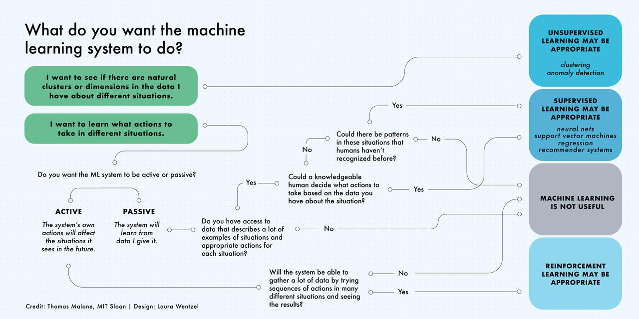


%3C%2Fmo%3E%3C%2Fmath%3E--%3E%3Cdefs%3E%3Cstyle%20type%3D%22text%2Fcss%22%3E%40font-face%7Bfont-family%3A'stix_italic1f4477bad7af3616c1f9'%3Bsrc%3Aurl(data%3Afont%2Ftruetype%3Bcharset%3Dutf-8%3Bbase64%2CAAEAAAAKAIAAAwAgT1MvMi7PBGUAAACsAAAATmNtYXCzVj0TAAAA%2FAAAADRnbHlmJRz6cgAAATAAAABlaGVhZAjbCH4AAAGYAAAANmhoZWEFzQfEAAAB0AAAACRobXR4MBdqngAAAfQAAAAIbG9jYQadRmQAAAH8AAAADG1heHAFYQCJAAACCAAAACBuYW1l%2FMdHqQAAAigAAAF7cG9zdAICAP8AAAOkAAAAIAAAAjsBkAAFAAAD6APoAAAAAAPoA%2BgAAAAAAAEA%2BgAAAAAAAAAAAAAAAAAAAAAAAAAAAAAAAAAAAAAgICAgAAAAINcbAwL%2FGgAAA%2F8BMQAAAAAAAgABAAEAAAAUAAMAAQAAABQABAAgAAAABAAEAAEAAAOf%2F%2F8AAAOf%2F%2F%2F8YgABAAAAAAACADz%2F7gK7ApsADwAfAAABFAYHBiMiJjU0Njc2MzYWBzQmIyIHDgEVFBYzMjc%2BAQK7c1xpbWN3Yk9wfWt2aUU8Y1c1PUM%2FXE47RgGia8Q%2BR3xuW8FFYQGGNEdRdUi2TlJXX0rWAAAAAAEAAAABAAAD7mBiXw889QADA%2Bj%2F%2F%2F%2F%2F0%2FxiZP%2F%2F%2F%2F%2FT%2FGJk%2FDb%2BzwWVA%2F8AAAAKAAIAAQAAAAAAAQAAA%2F%2F%2BzwAABcf8Nv4WBZUAAQAAAAAAAAAAAAAAAAAAAAIA%2BgAAAtIAPAAAAAAAAAAAAAAAZQABAAAAAgCGAAgAAAAAAAIAAAABAAEAAABAAAAAAAAAAAAAFQECAAAAAAAAAAEAFgAAAAAAAAAAAAIADgAWAAAAAAAAAAMAGAAkAAAAAAAAAAQAFgA8AAAAAAAAAAUAHABSAAAAAAAAAAYACwBuAAAAAAAAAAgAAAB5AAEAAAAAAAEAFgAAAAEAAAAAAAIADgAWAAEAAAAAAAMAGAAkAAEAAAAAAAQAFgA8AAEAAAAAAAUAHABSAAEAAAAAAAYACwBuAAEAAAAAAAgAAAB5AAMAAQQJAAEAFgAAAAMAAQQJAAIADgAWAAMAAQQJAAMAGAAkAAMAAQQJAAQAFgA8AAMAAQQJAAUAHABSAAMAAQQJAAYACwBuAAMAAQQJAAgAAAB5AFMAVABJAFgALQBJAHQAYQBsAGkAYwBSAGUAZwB1AGwAYQByACAAUwBUAEkAWAAtAEkAdABhAGwAaQBjAFMAVABJAFgALQBJAHQAYQBsAGkAYwBWAGUAcgBzAGkAbwBuACAAMQAuADEALgAxACBTVElYLUl0YWxpYwAAAwAAAAAAAAH%2FAP8AAAAAAAAAAAAAAAAAAAAAAAAAAA%3D%3D)format('truetype')%3Bfont-weight%3Anormal%3Bfont-style%3Anormal%3B%7D%40font-face%7Bfont-family%3A'stixc5b02a53929a0fc51d8f290bb80'%3Bsrc%3Aurl(data%3Afont%2Ftruetype%3Bcharset%3Dutf-8%3Bbase64%2CAAEAAAANAIAAAwBQT1MvMi8nBU0AAADcAAAATmNtYXDCjdaBAAABLAAAAERjdnQgSG4BcAAAAXAAAADYZnBnbUUgjnwAAAJIAAANbWdseWYcKO%2BSAAAPuAAAANdoZWFkDLPdGwAAEJAAAAA2aGhlYQjYEyQAABDIAAAAJGhtdHg0LeORAAAQ7AAAABBsb2NhTQ9wLwAAEPwAAAAUbWF4cBlhFX0AABEQAAAAIG5hbWV4T00CAAARMAAAAZ5wb3N0AgIA%2FwAAEtAAAAAgcHJlcFWzoI8AABLwAAAAvAAAApwBkAAFAAAD6APoAAAAAAPoA%2BgAAAAAAAEA%2BgAAAAAAAAAAAAAAAAAAAAAAAAAAAAAAAAAAAAAgICAgAAAAINf%2FAqX%2BvQAAA%2F8B5gAAAAAAAgABAAEAAAAUAAMAAQAAABQABAAwAAAACAAIAAIAAAAoACkAMf%2F%2FAAAAKAApADH%2F%2F%2F%2FZ%2F9n%2F0gABAAAAAAAAAAAAAAAAAAAAAAAAAAAAAAAAAAAAAAAAAAAAAAAAAAAAAAAAAAAAAAAAAAAAAABaAFoAHAAcApYAAAHCAAD%2FJwP%2F%2FhoCpP%2FyAcz%2F9v8mA%2F%2F%2BGgBZAFkAIAAgApYAAAKrAcL%2F9v8nA%2F%2F%2BGgKk%2F%2FICqwHM%2F%2Fb%2FJgP%2F%2FhoAWgBaABwAHAKWAAACqwHCAAD%2FJwP%2F%2FhoCpP%2FyAqsBzP%2F2%2FyYD%2F%2F4aAFoAWgAcABwClgEOAqsCOgFQ%2F%2BwD%2F%2F4aAqT%2F8gKrAjr%2F9v%2FsA%2F%2F%2BGgAYABgAGAAYA%2F%2F%2BGgP%2F%2FhqwACwgsABVWEVZICBLuAAOUUuwBlNaWLA0G7AoWWBmIIpVWLACJWG5CAAIAGNjI2IbISGwAFmwAEMjRLIAAQBDYEItsAEssCBgZi2wAiwgZCCwwFCwBCZasigBC0NFY0WwBkVYIbADJVlSW1ghIyEbilggsFBQWCGwQFkbILA4UFghsDhZWSCxAQtDRWNFYWSwKFBYIbEBC0NFY0UgsDBQWCGwMFkbILDAUFggZiCKimEgsApQWGAbILAgUFghsApgGyCwNlBYIbA2YBtgWVlZG7ACJbAKQ2OwAFJYsABLsApQWCGwCkMbS7AeUFghsB5LYbgQAGOwCkNjuAUAYllZZGFZsAErWVkjsABQWGVZWS2wAywgRSCwBCVhZCCwBUNQWLAFI0KwBiNCGyEhWbABYC2wBCwjISMhIGSxBWJCILAGI0KwBkVYG7EBC0NFY7EBC0OwBWBFY7ADKiEgsAZDIIogirABK7EwBSWwBCZRWGBQG2FSWVgjWSFZILBAU1iwASsbIbBAWSOwAFBYZVktsAUssAdDK7IAAgBDYEItsAYssAcjQiMgsAAjQmGwAmJmsAFjsAFgsAUqLbAHLCAgRSCwDENjuAQAYiCwAFBYsEBgWWawAWNgRLABYC2wCCyyBwwAQ0VCKiGyAAEAQ2BCLbAJLLAAQyNEsgABAENgQi2wCiwgIEUgsAErI7AAQ7AEJWAgRYojYSBkILAgUFghsAAbsDBQWLAgG7BAWVkjsABQWGVZsAMlI2FERLABYC2wCywgIEUgsAErI7AAQ7AEJWAgRYojYSBksCRQWLAAG7BAWSOwAFBYZVmwAyUjYUREsAFgLbAMLCCwACNCsgsKA0VYIRsjIVkqIS2wDSyxAgJFsGRhRC2wDiywAWAgILANQ0qwAFBYILANI0JZsA5DSrAAUlggsA4jQlktsA8sILAQYmawAWMguAQAY4ojYbAPQ2AgimAgsA8jQiMtsBAsS1RYsQRkRFkksA1lI3gtsBEsS1FYS1NYsQRkRFkbIVkksBNlI3gtsBIssQAQQ1VYsRAQQ7ABYUKwDytZsABDsAIlQrENAiVCsQ4CJUKwARYjILADJVBYsQEAQ2CwBCVCioogiiNhsA4qISOwAWEgiiNhsA4qIRuxAQBDYLACJUKwAiVhsA4qIVmwDUNHsA5DR2CwAmIgsABQWLBAYFlmsAFjILAMQ2O4BABiILAAUFiwQGBZZrABY2CxAAATI0SwAUOwAD6yAQEBQ2BCLbATLACxAAJFVFiwECNCIEWwDCNCsAsjsAVgQiBgsAFhtRISAQAPAEJCimCxEgYrsIkrGyJZLbAULLEAEystsBUssQETKy2wFiyxAhMrLbAXLLEDEystsBgssQQTKy2wGSyxBRMrLbAaLLEGEystsBsssQcTKy2wHCyxCBMrLbAdLLEJEystsCksIyCwEGJmsAFjsAZgS1RYIyAusAFdGyEhWS2wKiwjILAQYmawAWOwFmBLVFgjIC6wAXEbISFZLbArLCMgsBBiZrABY7AmYEtUWCMgLrABchshIVktsB4sALANK7EAAkVUWLAQI0IgRbAMI0KwCyOwBWBCIGCwAWG1EhIBAA8AQkKKYLESBiuwiSsbIlktsB8ssQAeKy2wICyxAR4rLbAhLLECHistsCIssQMeKy2wIyyxBB4rLbAkLLEFHistsCUssQYeKy2wJiyxBx4rLbAnLLEIHistsCgssQkeKy2wLCwgPLABYC2wLSwgYLASYCBDI7ABYEOwAiVhsAFgsCwqIS2wLiywLSuwLSotsC8sICBHICCwDENjuAQAYiCwAFBYsEBgWWawAWNgI2E4IyCKVVggRyAgsAxDY7gEAGIgsABQWLBAYFlmsAFjYCNhOBshWS2wMCwAsQACRVRYsQwLRUKwARawLyqxBQEVRVgwWRsiWS2wMSwAsA0rsQACRVRYsQwLRUKwARawLyqxBQEVRVgwWRsiWS2wMiwgNbABYC2wMywAsQwLRUKwAUVjuAQAYiCwAFBYsEBgWWawAWOwASuwDENjuAQAYiCwAFBYsEBgWWawAWOwASuwABa0AAAAAABEPiM4sTIBFSohLbA0LCA8IEcgsAxDY7gEAGIgsABQWLBAYFlmsAFjYLAAQ2E4LbA1LC4XPC2wNiwgPCBHILAMQ2O4BABiILAAUFiwQGBZZrABY2CwAENhsAFDYzgtsDcssQIAFiUgLiBHsAAjQrACJUmKikcjRyNhIFhiGyFZsAEjQrI2AQEVFCotsDgssAAWsBEjQrAEJbAEJUcjRyNhsQoAQrAJQytlii4jICA8ijgtsDkssAAWsBEjQrAEJbAEJSAuRyNHI2EgsAQjQrEKAEKwCUMrILBgUFggsEBRWLMCIAMgG7MCJgMaWUJCIyCwCEMgiiNHI0cjYSNGYLAEQ7ACYiCwAFBYsEBgWWawAWNgILABKyCKimEgsAJDYGQjsANDYWRQWLACQ2EbsANDYFmwAyWwAmIgsABQWLBAYFlmsAFjYSMgILAEJiNGYTgbI7AIQ0awAiWwCENHI0cjYWAgsARDsAJiILAAUFiwQGBZZrABY2AjILABKyOwBENgsAErsAUlYbAFJbACYiCwAFBYsEBgWWawAWOwBCZhILAEJWBkI7ADJWBkUFghGyMhWSMgILAEJiNGYThZLbA6LLAAFrARI0IgICCwBSYgLkcjRyNhIzw4LbA7LLAAFrARI0IgsAgjQiAgIEYjR7ABKyNhOC2wPCywABawESNCsAMlsAIlRyNHI2GwAFRYLiA8IyEbsAIlsAIlRyNHI2EgsAUlsAQlRyNHI2GwBiWwBSVJsAIlYbkIAAgAY2MjIFhiGyFZY7gEAGIgsABQWLBAYFlmsAFjYCMuIyAgPIo4IyFZLbA9LLAAFrARI0IgsAhDIC5HI0cjYSBgsCBgZrACYiCwAFBYsEBgWWawAWMjICA8ijgtsD4sIyAuRrACJUawEUNYUBtSWVggPFkusS4BFCstsD8sIyAuRrACJUawEUNYUhtQWVggPFkusS4BFCstsEAsIyAuRrACJUawEUNYUBtSWVggPFkjIC5GsAIlRrARQ1hSG1BZWCA8WS6xLgEUKy2wQSywOCsjIC5GsAIlRrARQ1hQG1JZWCA8WS6xLgEUKy2wQiywOSuKICA8sAQjQoo4IyAuRrACJUawEUNYUBtSWVggPFkusS4BFCuwBEMusC4rLbBDLLAAFrAEJbAEJiAgIEYjR2GwCiNCLkcjRyNhsAlDKyMgPCAuIzixLgEUKy2wRCyxCAQlQrAAFrAEJbAEJSAuRyNHI2EgsAQjQrEKAEKwCUMrILBgUFggsEBRWLMCIAMgG7MCJgMaWUJCIyBHsARDsAJiILAAUFiwQGBZZrABY2AgsAErIIqKYSCwAkNgZCOwA0NhZFBYsAJDYRuwA0NgWbADJbACYiCwAFBYsEBgWWawAWNhsAIlRmE4IyA8IzgbISAgRiNHsAErI2E4IVmxLgEUKy2wRSyxADgrLrEuARQrLbBGLLEAOSshIyAgPLAEI0IjOLEuARQrsARDLrAuKy2wRyywABUgR7AAI0KyAAEBFRQTLrA0Ki2wSCywABUgR7AAI0KyAAEBFRQTLrA0Ki2wSSyxAAEUE7A1Ki2wSiywNyotsEsssAAWRSMgLiBGiiNhOLEuARQrLbBMLLAII0KwSystsE0ssgAARCstsE4ssgABRCstsE8ssgEARCstsFAssgEBRCstsFEssgAARSstsFIssgABRSstsFMssgEARSstsFQssgEBRSstsFUsswAAAEErLbBWLLMAAQBBKy2wVyyzAQAAQSstsFgsswEBAEErLbBZLLMAAAFBKy2wWiyzAAEBQSstsFssswEAAUErLbBcLLMBAQFBKy2wXSyyAABDKy2wXiyyAAFDKy2wXyyyAQBDKy2wYCyyAQFDKy2wYSyyAABGKy2wYiyyAAFGKy2wYyyyAQBGKy2wZCyyAQFGKy2wZSyzAAAAQistsGYsswABAEIrLbBnLLMBAABCKy2waCyzAQEAQistsGksswAAAUIrLbBqLLMAAQFCKy2wayyzAQABQistsGwsswEBAUIrLbBtLLEAOisusS4BFCstsG4ssQA6K7A%2BKy2wbyyxADorsD8rLbBwLLAAFrEAOiuwQCstsHEssQE6K7A%2BKy2wciyxATorsD8rLbBzLLAAFrEBOiuwQCstsHQssQA7Ky6xLgEUKy2wdSyxADsrsD4rLbB2LLEAOyuwPystsHcssQA7K7BAKy2weCyxATsrsD4rLbB5LLEBOyuwPystsHossQE7K7BAKy2weyyxADwrLrEuARQrLbB8LLEAPCuwPistsH0ssQA8K7A%2FKy2wfiyxADwrsEArLbB%2FLLEBPCuwPistsIAssQE8K7A%2FKy2wgSyxATwrsEArLbCCLLEAPSsusS4BFCstsIMssQA9K7A%2BKy2whCyxAD0rsD8rLbCFLLEAPSuwQCstsIYssQE9K7A%2BKy2whyyxAT0rsD8rLbCILLEBPSuwQCstsIksswkEAgNFWCEbIyFZQiuwCGWwAyRQeLEFARVFWDBZLQAAAAABADD%2FTwEwAqQADAAGswYBATArBQcuATUQNxcOARUUFgEwDHSA9wlmREahEELogwEVkxBXqZWUuAABAB3%2FTwEdAqQADAAGswYBATArEzceARUQByc%2BATU0Jh0McoL3CWdDQwKUEETogf7vlxBVqZeYtwABAG8AAAGKAqQAEgAmQCMMCwIBAgFKDgECSAACAQKDAwEBAQBdAAAAQQBMGCQREAQJGCspATU%2BATURNCMiDwE1NxcRFBYzAYr%2B7DcoHg4fG7MJKDcPAyMqAcExDAoOWwP9qyEcAAABAAAAAQAAM5ipa18PPPUAAwPo%2F%2F%2F%2F%2F9RjTQ3%2F%2F%2F%2F%2F1GNNDfw2%2FhoIoAP%2FAAAACgACAAEAAAAAAAEAAAP%2F%2FhoAAAj4%2FDb9yQigAAEAAAAAAAAAAAAAAAAAAAAEAPoAAAFNADABTQAdAfQAbwAAAAAAAAAAAAAAOQAAAHIAAADXAAEAAAAEBwwBLQAAAAAAAgOIA5oAiwAABdgK1QAAAAAAAAAVAQIAAAAAAAAAAQAgAAAAAAAAAAAAAgAOACAAAAAAAAAAAwAiAC4AAAAAAAAABAAgAFAAAAAAAAAABQAcAHAAAAAAAAAABgAQAIwAAAAAAAAACAAAAJwAAQAAAAAAAQAgAAAAAQAAAAAAAgAOACAAAQAAAAAAAwAiAC4AAQAAAAAABAAgAFAAAQAAAAAABQAcAHAAAQAAAAAABgAQAIwAAQAAAAAACAAAAJwAAwABBAkAAQAgAAAAAwABBAkAAgAOACAAAwABBAkAAwAiAC4AAwABBAkABAAgAFAAAwABBAkABQAcAHAAAwABBAkABgAQAIwAAwABBAkACAAAAJwAUwBUAEkAWAAtAFIAZQBnAHUAbABhAHIALQBUAFQARgBSAGUAZwB1AGwAYQByACAAUwBUAEkAWAAtAFIAZQBnAHUAbABhAHIALQBUAFQARgBTAFQASQBYAC0AUgBlAGcAdQBsAGEAcgAtAFQAVABGAFYAZQByAHMAaQBvAG4AIAAxAC4AMQAuADEAIFNUSVgtUmVndWxhci1UVEYAAAADAAAAAAAAAf8A%2FwAAAAAAAAAAAAAAAAAAAAAAAAAAAEu4AMhSWLEBAY5ZsAG5CAAIAGNwsQAHQrYAX0s3IwUAKrEAB0JADGYCUgg%2BCCoIGAcFCCqxAAdCQAxqAFwGSAY0BiEFBQgqsQAMQr4ZwBTAD8AKwAZAAAUACSqxABFCvgBAAEAAQABAAEAABQAJKrEDAESxJAGIUViwQIhYsQMARLEmAYhRWLoIgAABBECIY1RYsQMARFlZWVlADGgCVAhACCwIGgcFDCq4Af%2BFsASNsQIARLMFZAYAREQ%3D)format('truetype')%3Bfont-weight%3Anormal%3Bfont-style%3Anormal%3B%7D%3C%2Fstyle%3E%3C%2Fdefs%3E%3Ctext%20font-family%3D%22stix_italic1f4477bad7af3616c1f9%22%20font-size%3D%2216%22%20text-anchor%3D%22middle%22%20x%3D%226.5%22%20y%3D%2216%22%3E%26%23x39F%3B%3C%2Ftext%3E%3Ctext%20font-family%3D%22stixc5b02a53929a0fc51d8f290bb80%22%20font-size%3D%2216%22%20text-anchor%3D%22middle%22%20x%3D%2217.5%22%20y%3D%2216%22%3E(%3C%2Ftext%3E%3Ctext%20font-family%3D%22stixc5b02a53929a0fc51d8f290bb80%22%20font-size%3D%2216%22%20text-anchor%3D%22middle%22%20x%3D%2226.5%22%20y%3D%2216%22%3E1%3C%2Ftext%3E%3Ctext%20font-family%3D%22stixc5b02a53929a0fc51d8f290bb80%22%20font-size%3D%2216%22%20text-anchor%3D%22middle%22%20x%3D%2233.5%22%20y%3D%2216%22%3E)%3C%2Ftext%3E%3C%2Fsvg%3E)
%3C%2Fmo%3E%3C%2Fmath%3E--%3E%3Cdefs%3E%3Cstyle%20type%3D%22text%2Fcss%22%3E%40font-face%7Bfont-family%3A'stix_italicb2af4cb567def0eaff20'%3Bsrc%3Aurl(data%3Afont%2Ftruetype%3Bcharset%3Dutf-8%3Bbase64%2CAAEAAAAKAIAAAwAgT1MvMi7PBGUAAACsAAAATmNtYXCzVj0TAAAA%2FAAAADxnbHlmJRz6cgAAATgAAAD3aGVhZAjbCH4AAAIwAAAANmhoZWEFzQfEAAACaAAAACRobXR4MBdqngAAAowAAAAMbG9jYQadRmQAAAKYAAAAEG1heHAFYQCJAAACqAAAACBuYW1l%2FMdHqQAAAsgAAAF7cG9zdAICAP8AAAREAAAAIAAAAjsBkAAFAAAD6APoAAAAAAPoA%2BgAAAAAAAEA%2BgAAAAAAAAAAAAAAAAAAAAAAAAAAAAAAAAAAAAAgICAgAAAAINcbAwL%2FGgAAA%2F8BMQAAAAAAAgABAAEAAAAUAAMAAQAAABQABAAoAAAABgAEAAEAAgBPAG7%2F%2FwAAAE8Abv%2F%2F%2F7L%2FlAABAAAAAAAAAAIAPP%2FuArsCmwAPAB8AAAEUBgcGIyImNTQ2NzYzNhYHNCYjIgcOARUUFjMyNz4BArtzXGltY3diT3B9a3ZpRTxjVzU9Qz9cTjtGAaJrxD5HfG5bwUVhAYY0R1F1SLZOUldfStYAAQAO%2F%2FcB2gG5ADEAACUXDgEjIiY1ND8BNjU0IyIGBw4BByMTNjU0Jic1PgE3Fwc%2BATMyFhUUDwEGFRQzMjc2AcwOMzYjFBsQLA4YHUUyIR8kS2ACGyYnYBsEQ0psMR8iCjgOEBMqB3UNRisbGxA7ojYZHUVJMU55AV4KBw8LARAIEQYC2nZmIRwZI8syCxI1CAAAAQAAAAEAAAPuYGJfDzz1AAMD6P%2F%2F%2F%2F%2FT%2FGJk%2F%2F%2F%2F%2F9P8YmT8Nv7PBZUD%2FwAAAAoAAgABAAAAAAABAAAD%2F%2F7PAAAFx%2Fw2%2FhYFlQABAAAAAAAAAAAAAAAAAAAAAwD6AAAC0gA8AfQADgAAAAAAAAAAAAAAZQAAAPcAAQAAAAMAhgAIAAAAAAACAAAAAQABAAAAQAAAAAAAAAAAABUBAgAAAAAAAAABABYAAAAAAAAAAAACAA4AFgAAAAAAAAADABgAJAAAAAAAAAAEABYAPAAAAAAAAAAFABwAUgAAAAAAAAAGAAsAbgAAAAAAAAAIAAAAeQABAAAAAAABABYAAAABAAAAAAACAA4AFgABAAAAAAADABgAJAABAAAAAAAEABYAPAABAAAAAAAFABwAUgABAAAAAAAGAAsAbgABAAAAAAAIAAAAeQADAAEECQABABYAAAADAAEECQACAA4AFgADAAEECQADABgAJAADAAEECQAEABYAPAADAAEECQAFABwAUgADAAEECQAGAAsAbgADAAEECQAIAAAAeQBTAFQASQBYAC0ASQB0AGEAbABpAGMAUgBlAGcAdQBsAGEAcgAgAFMAVABJAFgALQBJAHQAYQBsAGkAYwBTAFQASQBYAC0ASQB0AGEAbABpAGMAVgBlAHIAcwBpAG8AbgAgADEALgAxAC4AMQAgU1RJWC1JdGFsaWMAAAMAAAAAAAAB%2FwD%2FAAAAAAAAAAAAAAAAAAAAAAAAAAA%3D)format('truetype')%3Bfont-weight%3Anormal%3Bfont-style%3Anormal%3B%7D%40font-face%7Bfont-family%3A'stixc9c7656cb2e899b64d85a350450'%3Bsrc%3Aurl(data%3Afont%2Ftruetype%3Bcharset%3Dutf-8%3Bbase64%2CAAEAAAANAIAAAwBQT1MvMi8nBU0AAADcAAAATmNtYXDCjdaBAAABLAAAAERjdnQgSG4BcAAAAXAAAADYZnBnbUUgjnwAAAJIAAANbWdseWYcKO%2BSAAAPuAAAAVRoZWFkDLPdGwAAEQwAAAA2aGhlYQjYEyQAABFEAAAAJGhtdHg0LeORAAARaAAAABBsb2NhTQ9wLwAAEXgAAAAUbWF4cBlhFX0AABGMAAAAIG5hbWV4T00CAAARrAAAAZ5wb3N0AgIA%2FwAAE0wAAAAgcHJlcFWzoI8AABNsAAAAvAAAApwBkAAFAAAD6APoAAAAAAPoA%2BgAAAAAAAEA%2BgAAAAAAAAAAAAAAAAAAAAAAAAAAAAAAAAAAAAAgICAgAAAAINf%2FAqX%2BvQAAA%2F8B5gAAAAAAAgABAAEAAAAUAAMAAQAAABQABAAwAAAACAAIAAIAAAAoACkAM%2F%2F%2FAAAAKAApADP%2F%2F%2F%2FZ%2F9n%2F0AABAAAAAAAAAAAAAAAAAAAAAAAAAAAAAAAAAAAAAAAAAAAAAAAAAAAAAAAAAAAAAAAAAAAAAABaAFoAHAAcApYAAAHCAAD%2FJwP%2F%2FhoCpP%2FyAcz%2F9v8mA%2F%2F%2BGgBZAFkAIAAgApYAAAKrAcL%2F9v8nA%2F%2F%2BGgKk%2F%2FICqwHM%2F%2Fb%2FJgP%2F%2FhoAWgBaABwAHAKWAAACqwHCAAD%2FJwP%2F%2FhoCpP%2FyAqsBzP%2F2%2FyYD%2F%2F4aAFoAWgAcABwClgEOAqsCOgFQ%2F%2BwD%2F%2F4aAqT%2F8gKrAjr%2F9v%2FsA%2F%2F%2BGgAYABgAGAAYA%2F%2F%2BGgP%2F%2FhqwACwgsABVWEVZICBLuAAOUUuwBlNaWLA0G7AoWWBmIIpVWLACJWG5CAAIAGNjI2IbISGwAFmwAEMjRLIAAQBDYEItsAEssCBgZi2wAiwgZCCwwFCwBCZasigBC0NFY0WwBkVYIbADJVlSW1ghIyEbilggsFBQWCGwQFkbILA4UFghsDhZWSCxAQtDRWNFYWSwKFBYIbEBC0NFY0UgsDBQWCGwMFkbILDAUFggZiCKimEgsApQWGAbILAgUFghsApgGyCwNlBYIbA2YBtgWVlZG7ACJbAKQ2OwAFJYsABLsApQWCGwCkMbS7AeUFghsB5LYbgQAGOwCkNjuAUAYllZZGFZsAErWVkjsABQWGVZWS2wAywgRSCwBCVhZCCwBUNQWLAFI0KwBiNCGyEhWbABYC2wBCwjISMhIGSxBWJCILAGI0KwBkVYG7EBC0NFY7EBC0OwBWBFY7ADKiEgsAZDIIogirABK7EwBSWwBCZRWGBQG2FSWVgjWSFZILBAU1iwASsbIbBAWSOwAFBYZVktsAUssAdDK7IAAgBDYEItsAYssAcjQiMgsAAjQmGwAmJmsAFjsAFgsAUqLbAHLCAgRSCwDENjuAQAYiCwAFBYsEBgWWawAWNgRLABYC2wCCyyBwwAQ0VCKiGyAAEAQ2BCLbAJLLAAQyNEsgABAENgQi2wCiwgIEUgsAErI7AAQ7AEJWAgRYojYSBkILAgUFghsAAbsDBQWLAgG7BAWVkjsABQWGVZsAMlI2FERLABYC2wCywgIEUgsAErI7AAQ7AEJWAgRYojYSBksCRQWLAAG7BAWSOwAFBYZVmwAyUjYUREsAFgLbAMLCCwACNCsgsKA0VYIRsjIVkqIS2wDSyxAgJFsGRhRC2wDiywAWAgILANQ0qwAFBYILANI0JZsA5DSrAAUlggsA4jQlktsA8sILAQYmawAWMguAQAY4ojYbAPQ2AgimAgsA8jQiMtsBAsS1RYsQRkRFkksA1lI3gtsBEsS1FYS1NYsQRkRFkbIVkksBNlI3gtsBIssQAQQ1VYsRAQQ7ABYUKwDytZsABDsAIlQrENAiVCsQ4CJUKwARYjILADJVBYsQEAQ2CwBCVCioogiiNhsA4qISOwAWEgiiNhsA4qIRuxAQBDYLACJUKwAiVhsA4qIVmwDUNHsA5DR2CwAmIgsABQWLBAYFlmsAFjILAMQ2O4BABiILAAUFiwQGBZZrABY2CxAAATI0SwAUOwAD6yAQEBQ2BCLbATLACxAAJFVFiwECNCIEWwDCNCsAsjsAVgQiBgsAFhtRISAQAPAEJCimCxEgYrsIkrGyJZLbAULLEAEystsBUssQETKy2wFiyxAhMrLbAXLLEDEystsBgssQQTKy2wGSyxBRMrLbAaLLEGEystsBsssQcTKy2wHCyxCBMrLbAdLLEJEystsCksIyCwEGJmsAFjsAZgS1RYIyAusAFdGyEhWS2wKiwjILAQYmawAWOwFmBLVFgjIC6wAXEbISFZLbArLCMgsBBiZrABY7AmYEtUWCMgLrABchshIVktsB4sALANK7EAAkVUWLAQI0IgRbAMI0KwCyOwBWBCIGCwAWG1EhIBAA8AQkKKYLESBiuwiSsbIlktsB8ssQAeKy2wICyxAR4rLbAhLLECHistsCIssQMeKy2wIyyxBB4rLbAkLLEFHistsCUssQYeKy2wJiyxBx4rLbAnLLEIHistsCgssQkeKy2wLCwgPLABYC2wLSwgYLASYCBDI7ABYEOwAiVhsAFgsCwqIS2wLiywLSuwLSotsC8sICBHICCwDENjuAQAYiCwAFBYsEBgWWawAWNgI2E4IyCKVVggRyAgsAxDY7gEAGIgsABQWLBAYFlmsAFjYCNhOBshWS2wMCwAsQACRVRYsQwLRUKwARawLyqxBQEVRVgwWRsiWS2wMSwAsA0rsQACRVRYsQwLRUKwARawLyqxBQEVRVgwWRsiWS2wMiwgNbABYC2wMywAsQwLRUKwAUVjuAQAYiCwAFBYsEBgWWawAWOwASuwDENjuAQAYiCwAFBYsEBgWWawAWOwASuwABa0AAAAAABEPiM4sTIBFSohLbA0LCA8IEcgsAxDY7gEAGIgsABQWLBAYFlmsAFjYLAAQ2E4LbA1LC4XPC2wNiwgPCBHILAMQ2O4BABiILAAUFiwQGBZZrABY2CwAENhsAFDYzgtsDcssQIAFiUgLiBHsAAjQrACJUmKikcjRyNhIFhiGyFZsAEjQrI2AQEVFCotsDgssAAWsBEjQrAEJbAEJUcjRyNhsQoAQrAJQytlii4jICA8ijgtsDkssAAWsBEjQrAEJbAEJSAuRyNHI2EgsAQjQrEKAEKwCUMrILBgUFggsEBRWLMCIAMgG7MCJgMaWUJCIyCwCEMgiiNHI0cjYSNGYLAEQ7ACYiCwAFBYsEBgWWawAWNgILABKyCKimEgsAJDYGQjsANDYWRQWLACQ2EbsANDYFmwAyWwAmIgsABQWLBAYFlmsAFjYSMgILAEJiNGYTgbI7AIQ0awAiWwCENHI0cjYWAgsARDsAJiILAAUFiwQGBZZrABY2AjILABKyOwBENgsAErsAUlYbAFJbACYiCwAFBYsEBgWWawAWOwBCZhILAEJWBkI7ADJWBkUFghGyMhWSMgILAEJiNGYThZLbA6LLAAFrARI0IgICCwBSYgLkcjRyNhIzw4LbA7LLAAFrARI0IgsAgjQiAgIEYjR7ABKyNhOC2wPCywABawESNCsAMlsAIlRyNHI2GwAFRYLiA8IyEbsAIlsAIlRyNHI2EgsAUlsAQlRyNHI2GwBiWwBSVJsAIlYbkIAAgAY2MjIFhiGyFZY7gEAGIgsABQWLBAYFlmsAFjYCMuIyAgPIo4IyFZLbA9LLAAFrARI0IgsAhDIC5HI0cjYSBgsCBgZrACYiCwAFBYsEBgWWawAWMjICA8ijgtsD4sIyAuRrACJUawEUNYUBtSWVggPFkusS4BFCstsD8sIyAuRrACJUawEUNYUhtQWVggPFkusS4BFCstsEAsIyAuRrACJUawEUNYUBtSWVggPFkjIC5GsAIlRrARQ1hSG1BZWCA8WS6xLgEUKy2wQSywOCsjIC5GsAIlRrARQ1hQG1JZWCA8WS6xLgEUKy2wQiywOSuKICA8sAQjQoo4IyAuRrACJUawEUNYUBtSWVggPFkusS4BFCuwBEMusC4rLbBDLLAAFrAEJbAEJiAgIEYjR2GwCiNCLkcjRyNhsAlDKyMgPCAuIzixLgEUKy2wRCyxCAQlQrAAFrAEJbAEJSAuRyNHI2EgsAQjQrEKAEKwCUMrILBgUFggsEBRWLMCIAMgG7MCJgMaWUJCIyBHsARDsAJiILAAUFiwQGBZZrABY2AgsAErIIqKYSCwAkNgZCOwA0NhZFBYsAJDYRuwA0NgWbADJbACYiCwAFBYsEBgWWawAWNhsAIlRmE4IyA8IzgbISAgRiNHsAErI2E4IVmxLgEUKy2wRSyxADgrLrEuARQrLbBGLLEAOSshIyAgPLAEI0IjOLEuARQrsARDLrAuKy2wRyywABUgR7AAI0KyAAEBFRQTLrA0Ki2wSCywABUgR7AAI0KyAAEBFRQTLrA0Ki2wSSyxAAEUE7A1Ki2wSiywNyotsEsssAAWRSMgLiBGiiNhOLEuARQrLbBMLLAII0KwSystsE0ssgAARCstsE4ssgABRCstsE8ssgEARCstsFAssgEBRCstsFEssgAARSstsFIssgABRSstsFMssgEARSstsFQssgEBRSstsFUsswAAAEErLbBWLLMAAQBBKy2wVyyzAQAAQSstsFgsswEBAEErLbBZLLMAAAFBKy2wWiyzAAEBQSstsFssswEAAUErLbBcLLMBAQFBKy2wXSyyAABDKy2wXiyyAAFDKy2wXyyyAQBDKy2wYCyyAQFDKy2wYSyyAABGKy2wYiyyAAFGKy2wYyyyAQBGKy2wZCyyAQFGKy2wZSyzAAAAQistsGYsswABAEIrLbBnLLMBAABCKy2waCyzAQEAQistsGksswAAAUIrLbBqLLMAAQFCKy2wayyzAQABQistsGwsswEBAUIrLbBtLLEAOisusS4BFCstsG4ssQA6K7A%2BKy2wbyyxADorsD8rLbBwLLAAFrEAOiuwQCstsHEssQE6K7A%2BKy2wciyxATorsD8rLbBzLLAAFrEBOiuwQCstsHQssQA7Ky6xLgEUKy2wdSyxADsrsD4rLbB2LLEAOyuwPystsHcssQA7K7BAKy2weCyxATsrsD4rLbB5LLEBOyuwPystsHossQE7K7BAKy2weyyxADwrLrEuARQrLbB8LLEAPCuwPistsH0ssQA8K7A%2FKy2wfiyxADwrsEArLbB%2FLLEBPCuwPistsIAssQE8K7A%2FKy2wgSyxATwrsEArLbCCLLEAPSsusS4BFCstsIMssQA9K7A%2BKy2whCyxAD0rsD8rLbCFLLEAPSuwQCstsIYssQE9K7A%2BKy2whyyxAT0rsD8rLbCILLEBPSuwQCstsIksswkEAgNFWCEbIyFZQiuwCGWwAyRQeLEFARVFWDBZLQAAAAABADD%2FTwEwAqQADAAGswYBATArBQcuATUQNxcOARUUFgEwDHSA9wlmREahEELogwEVkxBXqZWUuAABAB3%2FTwEdAqQADAAGswYBATArEzceARUQByc%2BATU0Jh0McoL3CWdDQwKUEETogf7vlxBVqZeYtwABACn%2F8gGvAqQAKgBntyIJAQMEBQFKS7AXUFhAIwAEBQIFBAJ%2BAAIDAwJuAAUFAF8AAABISwADAwFgAAEBSQFMG0AkAAQFAgUEAn4AAgMFAgN8AAUFAF8AAABISwADAwFgAAEBSQFMWUAJJxUiIysjBgkaKxMnPgEzMhYVFAcWFxYUBw4BIyI1NDYzMhcWMzI2NTQnJiM1Njc2NTQmIyI9EBdiS0ZWXTccLC4if0dwGBEZJCwqN0toH0c4HFE5M1oB%2FgRLV0w9UjgYHTGgPC4vORAUGh9ZQHMeCg4TES5YMjQAAQAAAAEAADOYqWtfDzz1AAMD6P%2F%2F%2F%2F%2FUY00N%2F%2F%2F%2F%2F9RjTQ38Nv4aCKAD%2FwAAAAoAAgABAAAAAAABAAAD%2F%2F4aAAAI%2BPw2%2FckIoAABAAAAAAAAAAAAAAAAAAAABAD6AAABTQAwAU0AHQH0ACkAAAAAAAAAAAAAADkAAAByAAABVAABAAAABAcMAS0AAAAAAAIDiAOaAIsAAAXYCtUAAAAAAAAAFQECAAAAAAAAAAEAIAAAAAAAAAAAAAIADgAgAAAAAAAAAAMAIgAuAAAAAAAAAAQAIABQAAAAAAAAAAUAHABwAAAAAAAAAAYAEACMAAAAAAAAAAgAAACcAAEAAAAAAAEAIAAAAAEAAAAAAAIADgAgAAEAAAAAAAMAIgAuAAEAAAAAAAQAIABQAAEAAAAAAAUAHABwAAEAAAAAAAYAEACMAAEAAAAAAAgAAACcAAMAAQQJAAEAIAAAAAMAAQQJAAIADgAgAAMAAQQJAAMAIgAuAAMAAQQJAAQAIABQAAMAAQQJAAUAHABwAAMAAQQJAAYAEACMAAMAAQQJAAgAAACcAFMAVABJAFgALQBSAGUAZwB1AGwAYQByAC0AVABUAEYAUgBlAGcAdQBsAGEAcgAgAFMAVABJAFgALQBSAGUAZwB1AGwAYQByAC0AVABUAEYAUwBUAEkAWAAtAFIAZQBnAHUAbABhAHIALQBUAFQARgBWAGUAcgBzAGkAbwBuACAAMQAuADEALgAxACBTVElYLVJlZ3VsYXItVFRGAAAAAwAAAAAAAAH%2FAP8AAAAAAAAAAAAAAAAAAAAAAAAAAABLuADIUlixAQGOWbABuQgACABjcLEAB0K2AF9LNyMFACqxAAdCQAxmAlIIPggqCBgHBQgqsQAHQkAMagBcBkgGNAYhBQUIKrEADEK%2BGcAUwA%2FACsAGQAAFAAkqsQARQr4AQABAAEAAQABAAAUACSqxAwBEsSQBiFFYsECIWLEDAESxJgGIUVi6CIAAAQRAiGNUWLEDAERZWVlZQAxoAlQIQAgsCBoHBQwquAH%2FhbAEjbECAESzBWQGAERE)format('truetype')%3Bfont-weight%3Anormal%3Bfont-style%3Anormal%3B%7D%3C%2Fstyle%3E%3C%2Fdefs%3E%3Ctext%20font-family%3D%22stix_italicb2af4cb567def0eaff20%22%20font-size%3D%2216%22%20text-anchor%3D%22middle%22%20x%3D%226.5%22%20y%3D%2217%22%3EO%3C%2Ftext%3E%3Ctext%20font-family%3D%22stixc9c7656cb2e899b64d85a350450%22%20font-size%3D%2216%22%20text-anchor%3D%22middle%22%20x%3D%2217.5%22%20y%3D%2217%22%3E(%3C%2Ftext%3E%3Ctext%20font-family%3D%22stix_italicb2af4cb567def0eaff20%22%20font-size%3D%2216%22%20text-anchor%3D%22middle%22%20x%3D%2226.5%22%20y%3D%2217%22%3En%3C%2Ftext%3E%3Ctext%20font-family%3D%22stixc9c7656cb2e899b64d85a350450%22%20font-size%3D%2212%22%20text-anchor%3D%22middle%22%20x%3D%2235.5%22%20y%3D%2212%22%3E3%3C%2Ftext%3E%3Ctext%20font-family%3D%22stixc9c7656cb2e899b64d85a350450%22%20font-size%3D%2216%22%20text-anchor%3D%22middle%22%20x%3D%2241.5%22%20y%3D%2217%22%3E)%3C%2Ftext%3E%3C%2Fsvg%3E)
format('truetype')%3Bfont-weight%3Anormal%3Bfont-style%3Anormal%3B%7D%3C%2Fstyle%3E%3C%2Fdefs%3E%3Ctext%20font-family%3D%22stixd6bbe2bca03fef20fa280993226%22%20font-size%3D%2216%22%20text-anchor%3D%22middle%22%20x%3D%228.5%22%20y%3D%2218%22%3E10%3C%2Ftext%3E%3Ctext%20font-family%3D%22stixd6bbe2bca03fef20fa280993226%22%20font-size%3D%2212%22%20text-anchor%3D%22middle%22%20x%3D%2223.5%22%20y%3D%2212%22%3E10%3C%2Ftext%3E%3C%2Fsvg%3E)
format('truetype')%3Bfont-weight%3Anormal%3Bfont-style%3Anormal%3B%7D%3C%2Fstyle%3E%3C%2Fdefs%3E%3Ctext%20font-family%3D%22stix857c22a08fd528a8c7884f1cac5%22%20font-size%3D%2216%22%20text-anchor%3D%22middle%22%20x%3D%228.5%22%20y%3D%2218%22%3E10%3C%2Ftext%3E%3Ctext%20font-family%3D%22stix857c22a08fd528a8c7884f1cac5%22%20font-size%3D%2212%22%20text-anchor%3D%22middle%22%20x%3D%2223.5%22%20y%3D%2212%22%3E13%3C%2Ftext%3E%3C%2Fsvg%3E)
format('truetype')%3Bfont-weight%3Anormal%3Bfont-style%3Anormal%3B%7D%3C%2Fstyle%3E%3C%2Fdefs%3E%3Ctext%20font-family%3D%22stixa68ce141847af88b5c753071621%22%20font-size%3D%2216%22%20text-anchor%3D%22middle%22%20x%3D%228.5%22%20y%3D%2218%22%3E10%3C%2Ftext%3E%3Ctext%20font-family%3D%22stixa68ce141847af88b5c753071621%22%20font-size%3D%2212%22%20text-anchor%3D%22middle%22%20x%3D%2226.5%22%20y%3D%2212%22%3E284%3C%2Ftext%3E%3C%2Fsvg%3E)
format('truetype')%3Bfont-weight%3Anormal%3Bfont-style%3Anormal%3B%7D%3C%2Fstyle%3E%3C%2Fdefs%3E%3Ctext%20font-family%3D%22stixcaaf68eb9a2f3e53634c8da2bfe%22%20font-size%3D%2216%22%20text-anchor%3D%22middle%22%20x%3D%228.5%22%20y%3D%2218%22%3E10%3C%2Ftext%3E%3Ctext%20font-family%3D%22stixcaaf68eb9a2f3e53634c8da2bfe%22%20font-size%3D%2212%22%20text-anchor%3D%22middle%22%20x%3D%2229.5%22%20y%3D%2212%22%3E2993%3C%2Ftext%3E%3C%2Fsvg%3E)
%3C%2Fmo%3E%3C%2Fmath%3E--%3E%3Cdefs%3E%3Cstyle%20type%3D%22text%2Fcss%22%3E%40font-face%7Bfont-family%3A'stix_italic5f93f983524def3dca46'%3Bsrc%3Aurl(data%3Afont%2Ftruetype%3Bcharset%3Dutf-8%3Bbase64%2CAAEAAAAKAIAAAwAgT1MvMi7PBGUAAACsAAAATmNtYXCzVj0TAAAA%2FAAAADRnbHlmJRz6cgAAATAAAACSaGVhZAjbCH4AAAHEAAAANmhoZWEFzQfEAAAB%2FAAAACRobXR4MBdqngAAAiAAAAAIbG9jYQadRmQAAAIoAAAADG1heHAFYQCJAAACNAAAACBuYW1l%2FMdHqQAAAlQAAAF7cG9zdAICAP8AAAPQAAAAIAAAAjsBkAAFAAAD6APoAAAAAAPoA%2BgAAAAAAAEA%2BgAAAAAAAAAAAAAAAAAAAAAAAAAAAAAAAAAAAAAgICAgAAAAINcbAwL%2FGgAAA%2F8BMQAAAAAAAgABAAEAAAAUAAMAAQAAABQABAAgAAAABAAEAAEAAABu%2F%2F8AAABu%2F%2F%2F%2FkwABAAAAAAABAA7%2F9wHaAbkAMQAAJRcOASMiJjU0PwE2NTQjIgYHDgEHIxM2NTQmJzU%2BATcXBz4BMzIWFRQPAQYVFDMyNzYBzA4zNiMUGxAsDhgdRTIhHyRLYAIbJidgGwRDSmwxHyIKOA4QEyoHdQ1GKxsbEDuiNhkdRUkxTnkBXgoHDwsBEAgRBgLadmYhHBkjyzILEjUIAAAAAQAAAAEAAAPuYGJfDzz1AAMD6P%2F%2F%2F%2F%2FT%2FGJk%2F%2F%2F%2F%2F9P8YmT8Nv7PBZUD%2FwAAAAoAAgABAAAAAAABAAAD%2F%2F7PAAAFx%2Fw2%2FhYFlQABAAAAAAAAAAAAAAAAAAAAAgD6AAAB9AAOAAAAAAAAAAAAAACSAAEAAAACAIYACAAAAAAAAgAAAAEAAQAAAEAAAAAAAAAAAAAVAQIAAAAAAAAAAQAWAAAAAAAAAAAAAgAOABYAAAAAAAAAAwAYACQAAAAAAAAABAAWADwAAAAAAAAABQAcAFIAAAAAAAAABgALAG4AAAAAAAAACAAAAHkAAQAAAAAAAQAWAAAAAQAAAAAAAgAOABYAAQAAAAAAAwAYACQAAQAAAAAABAAWADwAAQAAAAAABQAcAFIAAQAAAAAABgALAG4AAQAAAAAACAAAAHkAAwABBAkAAQAWAAAAAwABBAkAAgAOABYAAwABBAkAAwAYACQAAwABBAkABAAWADwAAwABBAkABQAcAFIAAwABBAkABgALAG4AAwABBAkACAAAAHkAUwBUAEkAWAAtAEkAdABhAGwAaQBjAFIAZQBnAHUAbABhAHIAIABTAFQASQBYAC0ASQB0AGEAbABpAGMAUwBUAEkAWAAtAEkAdABhAGwAaQBjAFYAZQByAHMAaQBvAG4AIAAxAC4AMQAuADEAIFNUSVgtSXRhbGljAAADAAAAAAAAAf8A%2FwAAAAAAAAAAAAAAAAAAAAAAAAAA)format('truetype')%3Bfont-weight%3Anormal%3Bfont-style%3Anormal%3B%7D%40font-face%7Bfont-family%3A'stix5466fa8b9ba21cd7b7decf29c00'%3Bsrc%3Aurl(data%3Afont%2Ftruetype%3Bcharset%3Dutf-8%3Bbase64%2CAAEAAAANAIAAAwBQT1MvMi8nBU0AAADcAAAATmNtYXDCjdaBAAABLAAAAFRjdnQgSG4BcAAAAYAAAADYZnBnbUUgjnwAAAJYAAANbWdseWYcKO%2BSAAAPyAAAArJoZWFkDLPdGwAAEnwAAAA2aGhlYQjYEyQAABK0AAAAJGhtdHg0LeORAAAS2AAAABhsb2NhTQ9wLwAAEvAAAAAcbWF4cBlhFX0AABMMAAAAIG5hbWV4T00CAAATLAAAAZ5wb3N0AgIA%2FwAAFMwAAAAgcHJlcFWzoI8AABTsAAAAvAAAApwBkAAFAAAD6APoAAAAAAPoA%2BgAAAAAAAEA%2BgAAAAAAAAAAAAAAAAAAAAAAAAAAAAAAAAAAAAAgICAgAAAAINf%2FAqX%2BvQAAA%2F8B5gAAAAAAAgABAAEAAAAUAAMAAQAAABQABABAAAAADAAIAAIABAAoACkAZwBsAG%2F%2F%2FwAAACgAKQBnAGwAb%2F%2F%2F%2F9n%2F2f%2Bc%2F5j%2FlgABAAAAAAAAAAAAAAAAAAAAAAAAAAAAAAAAAAAAAAAAAAAAAAAAAAAAAAAAAAAAAAAAAAAAAAAAAAAAWgBaABwAHAKWAAABwgAA%2FycD%2F%2F4aAqT%2F8gHM%2F%2Fb%2FJgP%2F%2FhoAWQBZACAAIAKWAAACqwHC%2F%2Fb%2FJwP%2F%2FhoCpP%2FyAqsBzP%2F2%2FyYD%2F%2F4aAFoAWgAcABwClgAAAqsBwgAA%2FycD%2F%2F4aAqT%2F8gKrAcz%2F9v8mA%2F%2F%2BGgBaAFoAHAAcApYBDgKrAjoBUP%2FsA%2F%2F%2BGgKk%2F%2FICqwI6%2F%2Fb%2F7AP%2F%2FhoAGAAYABgAGAP%2F%2FhoD%2F%2F4asAAsILAAVVhFWSAgS7gADlFLsAZTWliwNBuwKFlgZiCKVViwAiVhuQgACABjYyNiGyEhsABZsABDI0SyAAEAQ2BCLbABLLAgYGYtsAIsIGQgsMBQsAQmWrIoAQtDRWNFsAZFWCGwAyVZUltYISMhG4pYILBQUFghsEBZGyCwOFBYIbA4WVkgsQELQ0VjRWFksChQWCGxAQtDRWNFILAwUFghsDBZGyCwwFBYIGYgiophILAKUFhgGyCwIFBYIbAKYBsgsDZQWCGwNmAbYFlZWRuwAiWwCkNjsABSWLAAS7AKUFghsApDG0uwHlBYIbAeS2G4EABjsApDY7gFAGJZWWRhWbABK1lZI7AAUFhlWVktsAMsIEUgsAQlYWQgsAVDUFiwBSNCsAYjQhshIVmwAWAtsAQsIyEjISBksQViQiCwBiNCsAZFWBuxAQtDRWOxAQtDsAVgRWOwAyohILAGQyCKIIqwASuxMAUlsAQmUVhgUBthUllYI1khWSCwQFNYsAErGyGwQFkjsABQWGVZLbAFLLAHQyuyAAIAQ2BCLbAGLLAHI0IjILAAI0JhsAJiZrABY7ABYLAFKi2wBywgIEUgsAxDY7gEAGIgsABQWLBAYFlmsAFjYESwAWAtsAgssgcMAENFQiohsgABAENgQi2wCSywAEMjRLIAAQBDYEItsAosICBFILABKyOwAEOwBCVgIEWKI2EgZCCwIFBYIbAAG7AwUFiwIBuwQFlZI7AAUFhlWbADJSNhRESwAWAtsAssICBFILABKyOwAEOwBCVgIEWKI2EgZLAkUFiwABuwQFkjsABQWGVZsAMlI2FERLABYC2wDCwgsAAjQrILCgNFWCEbIyFZKiEtsA0ssQICRbBkYUQtsA4ssAFgICCwDUNKsABQWCCwDSNCWbAOQ0qwAFJYILAOI0JZLbAPLCCwEGJmsAFjILgEAGOKI2GwD0NgIIpgILAPI0IjLbAQLEtUWLEEZERZJLANZSN4LbARLEtRWEtTWLEEZERZGyFZJLATZSN4LbASLLEAEENVWLEQEEOwAWFCsA8rWbAAQ7ACJUKxDQIlQrEOAiVCsAEWIyCwAyVQWLEBAENgsAQlQoqKIIojYbAOKiEjsAFhIIojYbAOKiEbsQEAQ2CwAiVCsAIlYbAOKiFZsA1DR7AOQ0dgsAJiILAAUFiwQGBZZrABYyCwDENjuAQAYiCwAFBYsEBgWWawAWNgsQAAEyNEsAFDsAA%2BsgEBAUNgQi2wEywAsQACRVRYsBAjQiBFsAwjQrALI7AFYEIgYLABYbUSEgEADwBCQopgsRIGK7CJKxsiWS2wFCyxABMrLbAVLLEBEystsBYssQITKy2wFyyxAxMrLbAYLLEEEystsBkssQUTKy2wGiyxBhMrLbAbLLEHEystsBwssQgTKy2wHSyxCRMrLbApLCMgsBBiZrABY7AGYEtUWCMgLrABXRshIVktsCosIyCwEGJmsAFjsBZgS1RYIyAusAFxGyEhWS2wKywjILAQYmawAWOwJmBLVFgjIC6wAXIbISFZLbAeLACwDSuxAAJFVFiwECNCIEWwDCNCsAsjsAVgQiBgsAFhtRISAQAPAEJCimCxEgYrsIkrGyJZLbAfLLEAHistsCAssQEeKy2wISyxAh4rLbAiLLEDHistsCMssQQeKy2wJCyxBR4rLbAlLLEGHistsCYssQceKy2wJyyxCB4rLbAoLLEJHistsCwsIDywAWAtsC0sIGCwEmAgQyOwAWBDsAIlYbABYLAsKiEtsC4ssC0rsC0qLbAvLCAgRyAgsAxDY7gEAGIgsABQWLBAYFlmsAFjYCNhOCMgilVYIEcgILAMQ2O4BABiILAAUFiwQGBZZrABY2AjYTgbIVktsDAsALEAAkVUWLEMC0VCsAEWsC8qsQUBFUVYMFkbIlktsDEsALANK7EAAkVUWLEMC0VCsAEWsC8qsQUBFUVYMFkbIlktsDIsIDWwAWAtsDMsALEMC0VCsAFFY7gEAGIgsABQWLBAYFlmsAFjsAErsAxDY7gEAGIgsABQWLBAYFlmsAFjsAErsAAWtAAAAAAARD4jOLEyARUqIS2wNCwgPCBHILAMQ2O4BABiILAAUFiwQGBZZrABY2CwAENhOC2wNSwuFzwtsDYsIDwgRyCwDENjuAQAYiCwAFBYsEBgWWawAWNgsABDYbABQ2M4LbA3LLECABYlIC4gR7AAI0KwAiVJiopHI0cjYSBYYhshWbABI0KyNgEBFRQqLbA4LLAAFrARI0KwBCWwBCVHI0cjYbEKAEKwCUMrZYouIyAgPIo4LbA5LLAAFrARI0KwBCWwBCUgLkcjRyNhILAEI0KxCgBCsAlDKyCwYFBYILBAUVizAiADIBuzAiYDGllCQiMgsAhDIIojRyNHI2EjRmCwBEOwAmIgsABQWLBAYFlmsAFjYCCwASsgiophILACQ2BkI7ADQ2FkUFiwAkNhG7ADQ2BZsAMlsAJiILAAUFiwQGBZZrABY2EjICCwBCYjRmE4GyOwCENGsAIlsAhDRyNHI2FgILAEQ7ACYiCwAFBYsEBgWWawAWNgIyCwASsjsARDYLABK7AFJWGwBSWwAmIgsABQWLBAYFlmsAFjsAQmYSCwBCVgZCOwAyVgZFBYIRsjIVkjICCwBCYjRmE4WS2wOiywABawESNCICAgsAUmIC5HI0cjYSM8OC2wOyywABawESNCILAII0IgICBGI0ewASsjYTgtsDwssAAWsBEjQrADJbACJUcjRyNhsABUWC4gPCMhG7ACJbACJUcjRyNhILAFJbAEJUcjRyNhsAYlsAUlSbACJWG5CAAIAGNjIyBYYhshWWO4BABiILAAUFiwQGBZZrABY2AjLiMgIDyKOCMhWS2wPSywABawESNCILAIQyAuRyNHI2EgYLAgYGawAmIgsABQWLBAYFlmsAFjIyAgPIo4LbA%2BLCMgLkawAiVGsBFDWFAbUllYIDxZLrEuARQrLbA%2FLCMgLkawAiVGsBFDWFIbUFlYIDxZLrEuARQrLbBALCMgLkawAiVGsBFDWFAbUllYIDxZIyAuRrACJUawEUNYUhtQWVggPFkusS4BFCstsEEssDgrIyAuRrACJUawEUNYUBtSWVggPFkusS4BFCstsEIssDkriiAgPLAEI0KKOCMgLkawAiVGsBFDWFAbUllYIDxZLrEuARQrsARDLrAuKy2wQyywABawBCWwBCYgICBGI0dhsAojQi5HI0cjYbAJQysjIDwgLiM4sS4BFCstsEQssQgEJUKwABawBCWwBCUgLkcjRyNhILAEI0KxCgBCsAlDKyCwYFBYILBAUVizAiADIBuzAiYDGllCQiMgR7AEQ7ACYiCwAFBYsEBgWWawAWNgILABKyCKimEgsAJDYGQjsANDYWRQWLACQ2EbsANDYFmwAyWwAmIgsABQWLBAYFlmsAFjYbACJUZhOCMgPCM4GyEgIEYjR7ABKyNhOCFZsS4BFCstsEUssQA4Ky6xLgEUKy2wRiyxADkrISMgIDywBCNCIzixLgEUK7AEQy6wListsEcssAAVIEewACNCsgABARUUEy6wNCotsEgssAAVIEewACNCsgABARUUEy6wNCotsEkssQABFBOwNSotsEossDcqLbBLLLAAFkUjIC4gRoojYTixLgEUKy2wTCywCCNCsEsrLbBNLLIAAEQrLbBOLLIAAUQrLbBPLLIBAEQrLbBQLLIBAUQrLbBRLLIAAEUrLbBSLLIAAUUrLbBTLLIBAEUrLbBULLIBAUUrLbBVLLMAAABBKy2wViyzAAEAQSstsFcsswEAAEErLbBYLLMBAQBBKy2wWSyzAAABQSstsFosswABAUErLbBbLLMBAAFBKy2wXCyzAQEBQSstsF0ssgAAQystsF4ssgABQystsF8ssgEAQystsGAssgEBQystsGEssgAARistsGIssgABRistsGMssgEARistsGQssgEBRistsGUsswAAAEIrLbBmLLMAAQBCKy2wZyyzAQAAQistsGgsswEBAEIrLbBpLLMAAAFCKy2waiyzAAEBQistsGssswEAAUIrLbBsLLMBAQFCKy2wbSyxADorLrEuARQrLbBuLLEAOiuwPistsG8ssQA6K7A%2FKy2wcCywABaxADorsEArLbBxLLEBOiuwPistsHIssQE6K7A%2FKy2wcyywABaxATorsEArLbB0LLEAOysusS4BFCstsHUssQA7K7A%2BKy2wdiyxADsrsD8rLbB3LLEAOyuwQCstsHgssQE7K7A%2BKy2weSyxATsrsD8rLbB6LLEBOyuwQCstsHsssQA8Ky6xLgEUKy2wfCyxADwrsD4rLbB9LLEAPCuwPystsH4ssQA8K7BAKy2wfyyxATwrsD4rLbCALLEBPCuwPystsIEssQE8K7BAKy2wgiyxAD0rLrEuARQrLbCDLLEAPSuwPistsIQssQA9K7A%2FKy2whSyxAD0rsEArLbCGLLEBPSuwPistsIcssQE9K7A%2FKy2wiCyxAT0rsEArLbCJLLMJBAIDRVghGyMhWUIrsAhlsAMkUHixBQEVRVgwWS0AAAAAAQAw%2F08BMAKkAAwABrMGAQEwKwUHLgE1EDcXDgEVFBYBMAx0gPcJZkRGoRBC6IMBFZMQV6mVlLgAAQAd%2F08BHQKkAAwABrMGAQEwKxM3HgEVEAcnPgE1NCYdDHKC9wlnQ0MClBBE6IH%2B75cQVamXmLcAAwAc%2FyYB1gHMAC8APQBLAI9ADCMJAgEGQxwCCAICSkuwFVBYQDEABgABAgYBZwAHBwRfAAQES0sAAAAFXQAFBUNLAAICCF8ACAhJSwAJCQNfAAMDTQNMG0AvAAUAAAYFAGUABgABAgYBZwAHBwRfAAQES0sAAgIIXwAICElLAAkJA18AAwNNA0xZQBNKSEJAPDo1My8tKiglNiQQCgkYKwEjFhUUBiMiLwEOARUUHwEeARUUBwYjIiY1NDY3LgE1NDc2Ny4BNTQ2MzIfARY7AQUVFBYzMjY1NCcmIyIGATQmIyInDgEVFBYzMjYB1lMTaDQLGxMUKE6BN0I8U3VIZSw2IBUuFxQyK2FGKCgWHRpN%2FsI5LiIoHhkwIycBGTdFYz8eE09CVWkBhCspTU4DAgYqDxcEBgI6LzovQDkoHDcnDxYQHSgTFRk%2BL0RfDwgKWQNIWTEpQjcvMv5CHBUNJCERISg1AAEAEwAAAQECqwATAChAJQsBAgECAQACAkoPDAIBSAABAgGDAAICAF0AAABBAEwYJxADCRcrISM1PgE1ETQmIyIHNTY3FxEUFhcBAewvHhIYFRBfPwUcLw8EHyoB1SQcAhAXFQT9sCobAwACAB3%2F9gHWAcwACwAZAB9AHAACAgFfAAEBS0sAAwMAXwAAAEwATCUlJCIECRgrJRQGIyImNTQ2MzIWBzQnJiMiBhUUFxYzMjYB1n1kXHx8ZV17WjIoNzRANSI4Nz%2FnaYiHZ2iAf4FyQDJVSoBNMmMAAAABAAAAAQAAM5ipa18PPPUAAwPo%2F%2F%2F%2F%2F9RjTQ3%2F%2F%2F%2F%2F1GNNDfw2%2FhoIoAP%2FAAAACgACAAEAAAAAAAEAAAP%2F%2FhoAAAj4%2FDb9yQigAAEAAAAAAAAAAAAAAAAAAAAGAPoAAAFNADABTQAdAfQAHAEWABMB9AAdAAAAAAAAAAAAAAA5AAAAcgAAAdgAAAJCAAACsgABAAAABgcMAS0AAAAAAAIDiAOaAIsAAAXYCtUAAAAAAAAAFQECAAAAAAAAAAEAIAAAAAAAAAAAAAIADgAgAAAAAAAAAAMAIgAuAAAAAAAAAAQAIABQAAAAAAAAAAUAHABwAAAAAAAAAAYAEACMAAAAAAAAAAgAAACcAAEAAAAAAAEAIAAAAAEAAAAAAAIADgAgAAEAAAAAAAMAIgAuAAEAAAAAAAQAIABQAAEAAAAAAAUAHABwAAEAAAAAAAYAEACMAAEAAAAAAAgAAACcAAMAAQQJAAEAIAAAAAMAAQQJAAIADgAgAAMAAQQJAAMAIgAuAAMAAQQJAAQAIABQAAMAAQQJAAUAHABwAAMAAQQJAAYAEACMAAMAAQQJAAgAAACcAFMAVABJAFgALQBSAGUAZwB1AGwAYQByAC0AVABUAEYAUgBlAGcAdQBsAGEAcgAgAFMAVABJAFgALQBSAGUAZwB1AGwAYQByAC0AVABUAEYAUwBUAEkAWAAtAFIAZQBnAHUAbABhAHIALQBUAFQARgBWAGUAcgBzAGkAbwBuACAAMQAuADEALgAxACBTVElYLVJlZ3VsYXItVFRGAAAAAwAAAAAAAAH%2FAP8AAAAAAAAAAAAAAAAAAAAAAAAAAABLuADIUlixAQGOWbABuQgACABjcLEAB0K2AF9LNyMFACqxAAdCQAxmAlIIPggqCBgHBQgqsQAHQkAMagBcBkgGNAYhBQUIKrEADEK%2BGcAUwA%2FACsAGQAAFAAkqsQARQr4AQABAAEAAQABAAAUACSqxAwBEsSQBiFFYsECIWLEDAESxJgGIUVi6CIAAAQRAiGNUWLEDAERZWVlZQAxoAlQIQAgsCBoHBQwquAH%2FhbAEjbECAESzBWQGAERE)format('truetype')%3Bfont-weight%3Anormal%3Bfont-style%3Anormal%3B%7D%3C%2Fstyle%3E%3C%2Fdefs%3E%3Ctext%20font-family%3D%22stix5466fa8b9ba21cd7b7decf29c00%22%20font-size%3D%2216%22%20text-anchor%3D%22middle%22%20x%3D%2210.5%22%20y%3D%2216%22%3Elog%3C%2Ftext%3E%3Ctext%20font-family%3D%22stix5466fa8b9ba21cd7b7decf29c00%22%20font-size%3D%2216%22%20text-anchor%3D%22middle%22%20x%3D%2224.5%22%20y%3D%2216%22%3E(%3C%2Ftext%3E%3Ctext%20font-family%3D%22stix_italic5f93f983524def3dca46%22%20font-size%3D%2216%22%20text-anchor%3D%22middle%22%20x%3D%2233.5%22%20y%3D%2216%22%3En%3C%2Ftext%3E%3Ctext%20font-family%3D%22stix5466fa8b9ba21cd7b7decf29c00%22%20font-size%3D%2216%22%20text-anchor%3D%22middle%22%20x%3D%2241.5%22%20y%3D%2216%22%3E)%3C%2Ftext%3E%3C%2Fsvg%3E)
format('truetype')%3Bfont-weight%3Anormal%3Bfont-style%3Anormal%3B%7D%40font-face%7Bfont-family%3A'stix9fd65e128874ec6b2ab01ec3155'%3Bsrc%3Aurl(data%3Afont%2Ftruetype%3Bcharset%3Dutf-8%3Bbase64%2CAAEAAAANAIAAAwBQT1MvMi8nBU0AAADcAAAATmNtYXDCjdaBAAABLAAAAExjdnQgSG4BcAAAAXgAAADYZnBnbUUgjnwAAAJQAAANbWdseWYcKO%2BSAAAPwAAAAsJoZWFkDLPdGwAAEoQAAAA2aGhlYQjYEyQAABK8AAAAJGhtdHg0LeORAAAS4AAAABRsb2NhTQ9wLwAAEvQAAAAYbWF4cBlhFX0AABMMAAAAIG5hbWV4T00CAAATLAAAAZ5wb3N0AgIA%2FwAAFMwAAAAgcHJlcFWzoI8AABTsAAAAvAAAApwBkAAFAAAD6APoAAAAAAPoA%2BgAAAAAAAEA%2BgAAAAAAAAAAAAAAAAAAAAAAAAAAAAAAAAAAAAAgICAgAAAAINf%2FAqX%2BvQAAA%2F8B5gAAAAAAAgABAAEAAAAUAAMAAQAAABQABAA4AAAACgAIAAIAAgAyAGcAbABv%2F%2F8AAAAyAGcAbABv%2F%2F%2F%2Fz%2F%2Bb%2F5f%2FlQABAAAAAAAAAAAAAAAAAAAAAAAAAAAAAAAAAAAAAAAAAAAAAAAAAAAAAAAAAAAAAAAAAAAAAAAAAFoAWgAcABwClgAAAcIAAP8nA%2F%2F%2BGgKk%2F%2FIBzP%2F2%2FyYD%2F%2F4aAFkAWQAgACAClgAAAqsBwv%2F2%2FycD%2F%2F4aAqT%2F8gKrAcz%2F9v8mA%2F%2F%2BGgBaAFoAHAAcApYAAAKrAcIAAP8nA%2F%2F%2BGgKk%2F%2FICqwHM%2F%2Fb%2FJgP%2F%2FhoAWgBaABwAHAKWAQ4CqwI6AVD%2F7AP%2F%2FhoCpP%2FyAqsCOv%2F2%2F%2BwD%2F%2F4aABgAGAAYABgD%2F%2F4aA%2F%2F%2BGrAALCCwAFVYRVkgIEu4AA5RS7AGU1pYsDQbsChZYGYgilVYsAIlYbkIAAgAY2MjYhshIbAAWbAAQyNEsgABAENgQi2wASywIGBmLbACLCBkILDAULAEJlqyKAELQ0VjRbAGRVghsAMlWVJbWCEjIRuKWCCwUFBYIbBAWRsgsDhQWCGwOFlZILEBC0NFY0VhZLAoUFghsQELQ0VjRSCwMFBYIbAwWRsgsMBQWCBmIIqKYSCwClBYYBsgsCBQWCGwCmAbILA2UFghsDZgG2BZWVkbsAIlsApDY7AAUliwAEuwClBYIbAKQxtLsB5QWCGwHkthuBAAY7AKQ2O4BQBiWVlkYVmwAStZWSOwAFBYZVlZLbADLCBFILAEJWFkILAFQ1BYsAUjQrAGI0IbISFZsAFgLbAELCMhIyEgZLEFYkIgsAYjQrAGRVgbsQELQ0VjsQELQ7AFYEVjsAMqISCwBkMgiiCKsAErsTAFJbAEJlFYYFAbYVJZWCNZIVkgsEBTWLABKxshsEBZI7AAUFhlWS2wBSywB0MrsgACAENgQi2wBiywByNCIyCwACNCYbACYmawAWOwAWCwBSotsAcsICBFILAMQ2O4BABiILAAUFiwQGBZZrABY2BEsAFgLbAILLIHDABDRUIqIbIAAQBDYEItsAkssABDI0SyAAEAQ2BCLbAKLCAgRSCwASsjsABDsAQlYCBFiiNhIGQgsCBQWCGwABuwMFBYsCAbsEBZWSOwAFBYZVmwAyUjYUREsAFgLbALLCAgRSCwASsjsABDsAQlYCBFiiNhIGSwJFBYsAAbsEBZI7AAUFhlWbADJSNhRESwAWAtsAwsILAAI0KyCwoDRVghGyMhWSohLbANLLECAkWwZGFELbAOLLABYCAgsA1DSrAAUFggsA0jQlmwDkNKsABSWCCwDiNCWS2wDywgsBBiZrABYyC4BABjiiNhsA9DYCCKYCCwDyNCIy2wECxLVFixBGREWSSwDWUjeC2wESxLUVhLU1ixBGREWRshWSSwE2UjeC2wEiyxABBDVVixEBBDsAFhQrAPK1mwAEOwAiVCsQ0CJUKxDgIlQrABFiMgsAMlUFixAQBDYLAEJUKKiiCKI2GwDiohI7ABYSCKI2GwDiohG7EBAENgsAIlQrACJWGwDiohWbANQ0ewDkNHYLACYiCwAFBYsEBgWWawAWMgsAxDY7gEAGIgsABQWLBAYFlmsAFjYLEAABMjRLABQ7AAPrIBAQFDYEItsBMsALEAAkVUWLAQI0IgRbAMI0KwCyOwBWBCIGCwAWG1EhIBAA8AQkKKYLESBiuwiSsbIlktsBQssQATKy2wFSyxARMrLbAWLLECEystsBcssQMTKy2wGCyxBBMrLbAZLLEFEystsBossQYTKy2wGyyxBxMrLbAcLLEIEystsB0ssQkTKy2wKSwjILAQYmawAWOwBmBLVFgjIC6wAV0bISFZLbAqLCMgsBBiZrABY7AWYEtUWCMgLrABcRshIVktsCssIyCwEGJmsAFjsCZgS1RYIyAusAFyGyEhWS2wHiwAsA0rsQACRVRYsBAjQiBFsAwjQrALI7AFYEIgYLABYbUSEgEADwBCQopgsRIGK7CJKxsiWS2wHyyxAB4rLbAgLLEBHistsCEssQIeKy2wIiyxAx4rLbAjLLEEHistsCQssQUeKy2wJSyxBh4rLbAmLLEHHistsCcssQgeKy2wKCyxCR4rLbAsLCA8sAFgLbAtLCBgsBJgIEMjsAFgQ7ACJWGwAWCwLCohLbAuLLAtK7AtKi2wLywgIEcgILAMQ2O4BABiILAAUFiwQGBZZrABY2AjYTgjIIpVWCBHICCwDENjuAQAYiCwAFBYsEBgWWawAWNgI2E4GyFZLbAwLACxAAJFVFixDAtFQrABFrAvKrEFARVFWDBZGyJZLbAxLACwDSuxAAJFVFixDAtFQrABFrAvKrEFARVFWDBZGyJZLbAyLCA1sAFgLbAzLACxDAtFQrABRWO4BABiILAAUFiwQGBZZrABY7ABK7AMQ2O4BABiILAAUFiwQGBZZrABY7ABK7AAFrQAAAAAAEQ%2BIzixMgEVKiEtsDQsIDwgRyCwDENjuAQAYiCwAFBYsEBgWWawAWNgsABDYTgtsDUsLhc8LbA2LCA8IEcgsAxDY7gEAGIgsABQWLBAYFlmsAFjYLAAQ2GwAUNjOC2wNyyxAgAWJSAuIEewACNCsAIlSYqKRyNHI2EgWGIbIVmwASNCsjYBARUUKi2wOCywABawESNCsAQlsAQlRyNHI2GxCgBCsAlDK2WKLiMgIDyKOC2wOSywABawESNCsAQlsAQlIC5HI0cjYSCwBCNCsQoAQrAJQysgsGBQWCCwQFFYswIgAyAbswImAxpZQkIjILAIQyCKI0cjRyNhI0ZgsARDsAJiILAAUFiwQGBZZrABY2AgsAErIIqKYSCwAkNgZCOwA0NhZFBYsAJDYRuwA0NgWbADJbACYiCwAFBYsEBgWWawAWNhIyAgsAQmI0ZhOBsjsAhDRrACJbAIQ0cjRyNhYCCwBEOwAmIgsABQWLBAYFlmsAFjYCMgsAErI7AEQ2CwASuwBSVhsAUlsAJiILAAUFiwQGBZZrABY7AEJmEgsAQlYGQjsAMlYGRQWCEbIyFZIyAgsAQmI0ZhOFktsDossAAWsBEjQiAgILAFJiAuRyNHI2EjPDgtsDsssAAWsBEjQiCwCCNCICAgRiNHsAErI2E4LbA8LLAAFrARI0KwAyWwAiVHI0cjYbAAVFguIDwjIRuwAiWwAiVHI0cjYSCwBSWwBCVHI0cjYbAGJbAFJUmwAiVhuQgACABjYyMgWGIbIVljuAQAYiCwAFBYsEBgWWawAWNgIy4jICA8ijgjIVktsD0ssAAWsBEjQiCwCEMgLkcjRyNhIGCwIGBmsAJiILAAUFiwQGBZZrABYyMgIDyKOC2wPiwjIC5GsAIlRrARQ1hQG1JZWCA8WS6xLgEUKy2wPywjIC5GsAIlRrARQ1hSG1BZWCA8WS6xLgEUKy2wQCwjIC5GsAIlRrARQ1hQG1JZWCA8WSMgLkawAiVGsBFDWFIbUFlYIDxZLrEuARQrLbBBLLA4KyMgLkawAiVGsBFDWFAbUllYIDxZLrEuARQrLbBCLLA5K4ogIDywBCNCijgjIC5GsAIlRrARQ1hQG1JZWCA8WS6xLgEUK7AEQy6wListsEMssAAWsAQlsAQmICAgRiNHYbAKI0IuRyNHI2GwCUMrIyA8IC4jOLEuARQrLbBELLEIBCVCsAAWsAQlsAQlIC5HI0cjYSCwBCNCsQoAQrAJQysgsGBQWCCwQFFYswIgAyAbswImAxpZQkIjIEewBEOwAmIgsABQWLBAYFlmsAFjYCCwASsgiophILACQ2BkI7ADQ2FkUFiwAkNhG7ADQ2BZsAMlsAJiILAAUFiwQGBZZrABY2GwAiVGYTgjIDwjOBshICBGI0ewASsjYTghWbEuARQrLbBFLLEAOCsusS4BFCstsEYssQA5KyEjICA8sAQjQiM4sS4BFCuwBEMusC4rLbBHLLAAFSBHsAAjQrIAAQEVFBMusDQqLbBILLAAFSBHsAAjQrIAAQEVFBMusDQqLbBJLLEAARQTsDUqLbBKLLA3Ki2wSyywABZFIyAuIEaKI2E4sS4BFCstsEwssAgjQrBLKy2wTSyyAABEKy2wTiyyAAFEKy2wTyyyAQBEKy2wUCyyAQFEKy2wUSyyAABFKy2wUiyyAAFFKy2wUyyyAQBFKy2wVCyyAQFFKy2wVSyzAAAAQSstsFYsswABAEErLbBXLLMBAABBKy2wWCyzAQEAQSstsFksswAAAUErLbBaLLMAAQFBKy2wWyyzAQABQSstsFwsswEBAUErLbBdLLIAAEMrLbBeLLIAAUMrLbBfLLIBAEMrLbBgLLIBAUMrLbBhLLIAAEYrLbBiLLIAAUYrLbBjLLIBAEYrLbBkLLIBAUYrLbBlLLMAAABCKy2wZiyzAAEAQistsGcsswEAAEIrLbBoLLMBAQBCKy2waSyzAAABQistsGosswABAUIrLbBrLLMBAAFCKy2wbCyzAQEBQistsG0ssQA6Ky6xLgEUKy2wbiyxADorsD4rLbBvLLEAOiuwPystsHAssAAWsQA6K7BAKy2wcSyxATorsD4rLbByLLEBOiuwPystsHMssAAWsQE6K7BAKy2wdCyxADsrLrEuARQrLbB1LLEAOyuwPistsHYssQA7K7A%2FKy2wdyyxADsrsEArLbB4LLEBOyuwPistsHkssQE7K7A%2FKy2weiyxATsrsEArLbB7LLEAPCsusS4BFCstsHwssQA8K7A%2BKy2wfSyxADwrsD8rLbB%2BLLEAPCuwQCstsH8ssQE8K7A%2BKy2wgCyxATwrsD8rLbCBLLEBPCuwQCstsIIssQA9Ky6xLgEUKy2wgyyxAD0rsD4rLbCELLEAPSuwPystsIUssQA9K7BAKy2whiyxAT0rsD4rLbCHLLEBPSuwPystsIgssQE9K7BAKy2wiSyzCQQCA0VYIRsjIVlCK7AIZbADJFB4sQUBFUVYMFktAAAAAAEAHQAAAdoCpAAbACpAJxsOAgMBAwEAAwJKAAEBAl8AAgJISwADAwBdAAAAQQBMJSUnEQQJGCslByE1Nz4BNTQmIyIGByc%2BATMyFhUUDwEzMjY3Ado2%2FnmyRjxKQTY%2FHhURZ1hTZoCl6iEnGImJDL1JekFDSjhKBV1qZExxh7AaKQADABz%2FJgHWAcwALwA9AEsAj0AMIwkCAQZDHAIIAgJKS7AVUFhAMQAGAAECBgFnAAcHBF8ABARLSwAAAAVdAAUFQ0sAAgIIXwAICElLAAkJA18AAwNNA0wbQC8ABQAABgUAZQAGAAECBgFnAAcHBF8ABARLSwACAghfAAgISUsACQkDXwADA00DTFlAE0pIQkA8OjUzLy0qKCU2JBAKCRgrASMWFRQGIyIvAQ4BFRQfAR4BFRQHBiMiJjU0NjcuATU0NzY3LgE1NDYzMh8BFjsBBRUUFjMyNjU0JyYjIgYBNCYjIicOARUUFjMyNgHWUxNoNAsbExQoToE3QjxTdUhlLDYgFS4XFDIrYUYoKBYdGk3%2BwjkuIigeGTAjJwEZN0VjPx4TT0JVaQGEKylNTgMCBioPFwQGAjovOi9AOSgcNycPFhAdKBMVGT4vRF8PCApZA0hZMSlCNy8y%2FkIcFQ0kIREhKDUAAQATAAABAQKrABMAKEAlCwECAQIBAAICSg8MAgFIAAECAYMAAgIAXQAAAEEATBgnEAMJFyshIzU%2BATURNCYjIgc1NjcXERQWFwEB7C8eEhgVEF8%2FBRwvDwQfKgHVJBwCEBcVBP2wKhsDAAIAHf%2F2AdYBzAALABkAH0AcAAICAV8AAQFLSwADAwBfAAAATABMJSUkIgQJGCslFAYjIiY1NDYzMhYHNCcmIyIGFRQXFjMyNgHWfWRcfHxlXXtaMig3NEA1Ijg3P%2BdpiIdnaIB%2FgXJAMlVKgE0yYwAAAAEAAAABAAAzmKlrXw889QADA%2Bj%2F%2F%2F%2F%2F1GNNDf%2F%2F%2F%2F%2FUY00N%2FDb%2BGgigA%2F8AAAAKAAIAAQAAAAAAAQAAA%2F%2F%2BGgAACPj8Nv3JCKAAAQAAAAAAAAAAAAAAAAAAAAUA%2BgAAAfQAHQH0ABwBFgATAfQAHQAAAAAAAAAAAAAAggAAAegAAAJSAAACwgABAAAABQcMAS0AAAAAAAIDiAOaAIsAAAXYCtUAAAAAAAAAFQECAAAAAAAAAAEAIAAAAAAAAAAAAAIADgAgAAAAAAAAAAMAIgAuAAAAAAAAAAQAIABQAAAAAAAAAAUAHABwAAAAAAAAAAYAEACMAAAAAAAAAAgAAACcAAEAAAAAAAEAIAAAAAEAAAAAAAIADgAgAAEAAAAAAAMAIgAuAAEAAAAAAAQAIABQAAEAAAAAAAUAHABwAAEAAAAAAAYAEACMAAEAAAAAAAgAAACcAAMAAQQJAAEAIAAAAAMAAQQJAAIADgAgAAMAAQQJAAMAIgAuAAMAAQQJAAQAIABQAAMAAQQJAAUAHABwAAMAAQQJAAYAEACMAAMAAQQJAAgAAACcAFMAVABJAFgALQBSAGUAZwB1AGwAYQByAC0AVABUAEYAUgBlAGcAdQBsAGEAcgAgAFMAVABJAFgALQBSAGUAZwB1AGwAYQByAC0AVABUAEYAUwBUAEkAWAAtAFIAZQBnAHUAbABhAHIALQBUAFQARgBWAGUAcgBzAGkAbwBuACAAMQAuADEALgAxACBTVElYLVJlZ3VsYXItVFRGAAAAAwAAAAAAAAH%2FAP8AAAAAAAAAAAAAAAAAAAAAAAAAAABLuADIUlixAQGOWbABuQgACABjcLEAB0K2AF9LNyMFACqxAAdCQAxmAlIIPggqCBgHBQgqsQAHQkAMagBcBkgGNAYhBQUIKrEADEK%2BGcAUwA%2FACsAGQAAFAAkqsQARQr4AQABAAEAAQABAAAUACSqxAwBEsSQBiFFYsECIWLEDAESxJgGIUVi6CIAAAQRAiGNUWLEDAERZWVlZQAxoAlQIQAgsCBoHBQwquAH%2FhbAEjbECAESzBWQGAERE)format('truetype')%3Bfont-weight%3Anormal%3Bfont-style%3Anormal%3B%7D%3C%2Fstyle%3E%3C%2Fdefs%3E%3Ctext%20font-family%3D%22stix9fd65e128874ec6b2ab01ec3155%22%20font-size%3D%2216%22%20text-anchor%3D%22middle%22%20x%3D%2210.5%22%20y%3D%2216%22%3Elog%3C%2Ftext%3E%3Ctext%20font-family%3D%22stix9fd65e128874ec6b2ab01ec3155%22%20font-size%3D%2212%22%20text-anchor%3D%22middle%22%20x%3D%2224.5%22%20y%3D%2224%22%3E2%3C%2Ftext%3E%3Ctext%20font-family%3D%22stix_italic5f93f983524def3dca46%22%20font-size%3D%2216%22%20text-anchor%3D%22middle%22%20x%3D%2231.5%22%20y%3D%2216%22%3En%3C%2Ftext%3E%3C%2Fsvg%3E)